US Index Prediction: A Multi-Index Framework for DJIA, S&P 500, and NAS100

Project Roadmap

Phase	Description	Status
Phase 1	Literature Review	Complete
Phase 2	Data Collection & Feature Engineering 7 gap studies completed — see Section 6 for full results.	Complete
Phase 3	Model Development & Backtesting Dual-system: Short specialist +$127,633 (PF 1.90, Run 3L). Dip-buy long model +$4,683 (PF 1.16, Run 3N, first profitable longs). 13 runs documented. See Sections 7.5-7.14.	In Progress
Phase 4	Walk-Forward Validation	Planned

1. Introduction

The three dominant US equity indices — the Dow Jones Industrial Average (DJIA, traded as US30), the S&P 500 (US500), and the NASDAQ-100 (NAS100) — are often treated as interchangeable proxies for "the US stock market." In practice, they differ profoundly in construction methodology, sector composition, and constituent overlap. The DJIA is price-weighted across 30 blue-chip stocks; the S&P 500 is float-adjusted market-cap-weighted across roughly 500 companies; the NAS100 is modified market-cap-weighted across 100 non-financial firms with heavy technology exposure. These structural differences create persistent, non-trivial divergences in short-horizon returns that are largely absent from the academic literature.

Most published research on US equity index prediction treats each index in isolation: momentum strategies on the S&P 500, mean-reversion on the DJIA, or machine learning forecasts for the NASDAQ. The cross-index dimension — how information propagates between the three indices, how their spreads behave across market regimes, and whether structural differences create exploitable signals — remains substantially understudied. This is surprising given that the futures on these three indices (ES, YM, NQ) are among the most liquid instruments in the world, and that relative-value trades between them are a staple of institutional desks (CME Group, "Stock Index Spread Opportunities").

This project aims to fill that gap. We begin with a comprehensive literature review covering cross-index dynamics, multi-index trading strategies, and structural differences that create tradeable opportunities. We then identify specific research gaps — several of which appear to be entirely unstudied in the academic literature — and outline a phased research plan to test them empirically. The data constraint is deliberate: we restrict ourselves to OHLCV data at minute resolution from MetaTrader 5, ensuring that any findings are reproducible without proprietary data feeds.

2. Cross-Index Dynamics

2.1 Lead-Lag Relationships

The foundational work on lead-lag in equity markets comes from Lo and MacKinlay (1990), who documented that returns of large-capitalisation stocks lead returns of smaller stocks, attributing the effect partly to nonsynchronous trading and partly to differential speed of adjustment to information. Chordia and Swaminathan (2000) refined this finding by showing that high-volume portfolios lead low-volume portfolios at daily and weekly horizons, even after controlling for firm size. The mechanism is not purely mechanical: high-volume stocks adjust faster to market-wide information because they attract more attention from informed traders and algorithmic market makers.

In the futures-spot domain, the evidence is decisive. Stoll and Whaley (1990) found that S&P 500 and Major Market Index futures returns lead the corresponding cash indices by approximately five minutes on average, with occasional leads exceeding ten minutes. Lower transaction costs, leverage, and the ease of short-selling in futures explain why price discovery concentrates there. Hasbrouck (2003) quantified this precisely: roughly 90% of price discovery in the S&P 500 occurs in E-mini futures (information share IS = 0.89 to 0.93). For the NASDAQ-100, E-mini futures similarly dominate. The SPY ETF contributes to sector ETF price discovery, but not the reverse.

At the tick level, Huth and Abergel (2011) demonstrated that the most liquid assets lead smaller and less liquid stocks, and that the lead-lag structure is not constant intraday but shows seasonality around macroeconomic announcements and the US market open. By the early 2020s, median lead-lag durations in major equity markets have compressed to under ten milliseconds.

Despite this extensive literature on futures-spot and large-small cap lead-lag, direct studies of information flow between the three major US equity indices are sparse. Because the DJIA contains only 30 price-weighted stocks while the NAS100 is technology-heavy and the S&P 500 is broadly cap-weighted, differential information absorption speeds should exist during sector-specific news events. For instance, technology earnings may move the NAS100 first, with the signal propagating to the S&P 500 and the DJIA lagging if the relevant stocks carry low price-weighting in the Dow. This hypothesis has not been formally tested.

2.2 Correlation Structure and Regime Dependence

Engle (2002) introduced the Dynamic Conditional Correlation (DCC-GARCH) framework, which has become the standard tool for estimating time-varying correlations between financial assets. The model proceeds in two stages: univariate GARCH for each series, followed by a parsimonious correlation model on the standardised residuals. For any study of cross-index dynamics, DCC-GARCH provides the natural starting point for measuring how tightly the three indices co-move and whether that co-movement is stable.

A critical methodological insight comes from Forbes and Rigobon (2002), who demonstrated that raw correlation coefficients are biased upward during high-volatility periods. After adjusting for this bias, they found no significant increase in unconditional correlation during the 1997 Asian crisis, the 1994 Mexican devaluation, or the 1987 US crash. What appeared to be crisis-driven contagion was in fact pre-existing interdependence made visible by elevated variance. This finding has direct implications for anyone studying cross-index correlation during stress periods: naive rolling correlations will systematically overstate the degree of regime change.

Hamilton (1989) introduced the Markov-switching model for macroeconomic time series, where model parameters depend on an unobservable regime variable that follows a first-order Markov chain. This framework underpins all subsequent regime-switching work in finance. Ang and Bekaert (2002) applied it to portfolio choice, documenting that correlations and volatilities increase in bear markets. Despite this, diversification retains value even under regime switching because the increase in correlation is not perfect.

Regarding the three indices specifically, a Nasdaq (2020) white paper documents that NAS100 correlation with DJIA and S&P 500 was weakest during the Tech Bubble and the low-volatility period of 2017, and strongest during and after the 2008 Financial Crisis. In low-volatility environments, correlations decline naturally as there is no strong macroeconomic signal forcing co-movement. Fry-McKibbin and Hsiao (2018) applied Markov-switching models to US indices and identified three regimes — tranquil, volatile, and turbulent — with the tranquil regime being most frequent, the volatile regime dominating 2008, and the turbulent regime dominating the first four months of 2020.

2.3 Sector Rotation Patterns

The three indices differ structurally in sector exposure. The DJIA tilts toward industrials, healthcare, consumer staples, and financials. The S&P 500 has approximately 30% technology, 13% healthcare, and 13% financials. The NAS100 is roughly 45% technology with significant communications and consumer discretionary exposure, but excludes financials entirely and has minimal energy and utilities representation. These are not minor differences: they mean that sector rotation directly translates into cross-index relative performance.

Barberis and Shleifer (2003) formalised this intuition in their style investing framework. They showed that investors categorise assets into styles and allocate capital at the category level rather than the individual-asset level. Assets within the same style co-move excessively; assets in different styles co-move too little relative to fundamentals. Importantly, style-level momentum and value strategies are more profitable than their asset-level counterparts. This framework maps directly onto the DJIA (value/industrial style) versus NAS100 (growth/technology style) distinction.

Moskowitz and Grinblatt (1999) found that industry momentum is highly profitable even after controlling for size, book-to-market, and individual stock momentum. The sector composition differences across the three indices create natural momentum and rotation opportunities. The 2025 to 2026 "Great Rotation" provides a real-time illustration: capital shifted from technology (NAS100 underperformed the S&P 500 by approximately 6% year-to-date in 2025) into financials, industrials, energy, and precious metals, with the DJIA outperforming as traditional sectors led.

2.4 Dispersion and Convergence Dynamics

The dispersion trading literature, reviewed by Drechsler, Moreira, and Savov (2018), documents that implied correlation among index constituents tends to exceed realised correlation. The core dispersion trade — buying straddles on individual stocks and selling straddles on the index — exploits this wedge. A study on S&P 500 constituents from 2000 to 2017 found statistically significant returns of 14.5% to 26.5% per annum after transaction costs. Dispersion trades are concave in correlation: they profit when individual stocks diverge and lose during stress periods when correlation spikes, making them inherently short the volatility of correlation.

While traditional dispersion trading operates at the single-stock versus index level, the concept extends naturally to a three-index framework. If the three indices are temporarily dislocated — for example, the NAS100 rallying while the DJIA falls — a convergence trade betting on mean-reversion of the spread exploits the same correlation premium at the index level.

2.5 Index Arbitrage and Constituent Overlap

The overlap structure between the three indices is asymmetric. All 30 DJIA stocks are constituents of the S&P 500 (100% overlap). Approximately 79 of the 100 NAS100 stocks also appear in the S&P 500. However, only six stocks appear in all three indices. Roughly 20% of DJIA weight maps to about 30% of NAS100 weight. This partial overlap means that the indices are neither independent nor identical — they share enough common constituents to co-move, but differ enough to diverge meaningfully during sector-specific events.

Greenwood and Sammon (2023) documented that the index inclusion/exclusion effect has diminished over time as passive investing has grown, but that discretionary S&P 500 deletions still beat additions by 22% in the following year. Index fund long-short rebalancing portfolios continue to earn 4.61% annualised. Each index follows its own rebalancing calendar: the S&P 500 rebalances quarterly with ad hoc additions, the DJIA changes infrequently at the committee's discretion, and the NAS100 rebalances annually in December with special rebalancing triggered when the largest stock exceeds 24% weight. These rebalancing events create predictable flow demands that can temporarily dislocate cross-index relationships.

3. Multi-Index Strategies in the Literature

3.1 Pairs and Spread Trading

Gatev, Goetzmann, and Rouwenhorst (2006) established the academic foundation for pairs trading. Using minimum-distance matching on normalised prices across the period 1962 to 2002, they found that a simple two-standard-deviation divergence trigger yielded average annualised excess returns of up to 11% for self-financing portfolios. More recently, Zhu (2024) found that trading cointegrated near-parity pairs generates 58 basis points per month after costs, with 71% convergence probability, outperforming distance-based selection methods.

Applied to index spreads, CME Group details the methodology for constructing intermarket spreads between ES, YM, and NQ futures. A trader who believes technology is overvalued relative to the broad market sells NQ and buys ES, capturing relative sector performance without directional exposure. These spreads benefit from reduced margin requirements (as low as 10% of outright) reflecting their lower risk profile.

3.2 Time-Series Momentum and Rotation

Moskowitz, Ooi, and Pedersen (2012) documented significant time-series momentum across 58 liquid instruments including equity index futures. A diversified time-series momentum (TSMOM) portfolio delivers substantial abnormal returns and performs best during extreme market moves. Applied to a three-index rotation framework — allocating to the index with the strongest trailing momentum at each rebalancing point — this is one of the most robust findings in quantitative finance, yet its specific application to DJIA/S&P 500/NAS100 rotation is untested.

Barberis and Shleifer (2003) showed that style rotation is more profitable than individual asset rotation. The DJIA-as-value versus NAS100-as-growth mapping provides a natural style rotation pair. Rothe (2023) formalised sector rotation using macroeconomic indicators to time sector ETF allocation, while Mamais (2025) showed that momentum profitability varies across sectors and time, with macroeconomic conditions predicting these shifts.

3.3 Risk-On/Risk-Off Regime Detection

Chari, Stedman, and Lundblad (2025) proposed a composite risk-on/risk-off (RORO) index using credit spreads, equity returns, implied volatility, funding liquidity, and currency/gold signals. NBER Working Paper 31907 (2023) argues for measuring RORO as a combination of risk aversion (the price of risk) and macroeconomic uncertainty (the quantity of risk). Li (2025) found that the largest negative VIX-to-S&P 500 correlation occurs when both markets are in a high-volatility state, a result directly applicable to regime-conditional hedging.

A particularly promising signal, used by practitioners but never formally studied, is the NAS100/DJIA ratio as a risk-on/risk-off indicator. When the NAS100 outperforms the DJIA, capital is flowing into growth and technology stocks, signalling risk-on conditions. When the DJIA outperforms the NAS100, capital is rotating into value and defensive sectors, signalling risk-off. The 2025 to 2026 "Great Rotation" episodes provide vivid real-time illustrations of this dynamic. Despite its widespread use on trading desks, no academic study has validated the NAS100/DJIA ratio as a regime indicator or tested whether conditioning on it improves strategy selection.

4. Research Gaps Identified

Our literature review reveals several research gaps, ranging from entirely unstudied phenomena to well-known effects that have never been rigorously validated on this specific set of instruments. We restrict attention to gaps that can be tested with OHLCV data at minute resolution — the data we have available from MetaTrader 5. The following four gaps carry the highest combination of novelty, feasibility, and practical value.

4.1 Price-Weighted vs. Cap-Weighted Divergence Signal

The DJIA is the only major US equity index that uses price-weighting. This construction methodology creates mechanical, non-fundamental divergences from cap-weighted indices around stock splits, constituent additions and deletions, and divisor adjustments. A stock split, which is economically neutral, changes a company's DJIA weight but has no effect on its S&P 500 or NAS100 weight. Passive DJIA-tracking funds must rebalance in response; S&P 500 and NAS100 trackers do not.

No published study has systematically tested this divergence as a mean-reversion trading signal. The weighting methodology difference is structural and permanent — it cannot be arbitraged away because it stems from index construction rules, not from mispricing. The divergence is directly observable as the spread between normalised US30 and US500 (or NAS100) price series, making it testable with standard OHLCV data. The planned methodology involves constructing the normalised spread, testing z-score mean-reversion entry and exit thresholds, identifying whether divergence events cluster around known structural events, and validating out of sample with walk-forward windows.

4.2 Trivariate Cointegration Regime Model

Most cointegration studies in the pairs-trading literature test bivariate relationships (e.g., SPY/IWM). However, the Johansen (1991) multivariate vector error correction model (VECM) framework allows testing cointegration among all three indices simultaneously. Trivariate cointegration can reveal cointegrating vectors that no bivariate test would detect — relationships where the three-way spread mean-reverts even though no two-way spread does.

Furthermore, no study examines how trivariate cointegration stability changes across market regimes. Cointegration can break down during crisis periods or structural breaks. A Markov-switching VECM that detects regime transitions and adjusts trading rules accordingly would be a novel contribution. The planned methodology involves Johansen trace and eigenvalue tests at multiple timeframes (M5, M15, H1, D1), estimation of cointegrating vectors and error-correction speeds, and regime-switching models to detect when cointegration breaks down.

4.3 NAS100/DJIA Ratio as a Regime Indicator

As discussed in Section 3.3, the NAS100/DJIA ratio is widely used by practitioners as a risk-on/risk-off proxy, but it has never been formally validated. Zero academic studies exist. The planned empirical work will construct the ratio time series, define regimes based on the direction and magnitude of ratio changes across multiple lookback windows, and test whether regime identification predicts which index has the highest forward returns, whether momentum or mean-reversion strategies perform better in each regime, and whether volatility is expanding or contracting. The 2025 to 2026 "Great Rotation" provides a natural out-of-sample test period.

4.4 Cross-Index Lead-Lag at Minute Frequency

The academic lead-lag literature focuses on futures versus spot or large-cap versus small-cap stocks. No study directly measures information flow between US30, US500, and NAS100 at minute frequency, conditional on the type of move. During sector-specific events, differential absorption speeds should exist: technology earnings may move the NAS100 first, with the signal propagating to the S&P 500 and reaching the DJIA last. The planned methodology involves Granger causality tests at lags of one to ten minutes, time-varying lead-lag estimation via rolling window cross-correlation, conditioning on volatility regime and time of day, and testing whether detected lead-lag patterns are exploitable after spread costs.

4.5 Additional Gaps

Beyond the four primary gaps, our review identified several secondary opportunities:

• DJIA stock-split event arbitrage — when a DJIA constituent splits, its index weight drops mechanically while its weight in the S&P 500 and NAS100 is unaffected, creating a multi-index relative-value window that has never been formally studied.
• Joint multi-index Hidden Markov Model — most HMMs in the financial literature use single-index returns; a joint HMM on all three indices could capture cross-index states such as "technology-led rally," "broad selloff," "sector rotation," or "convergence."
• Anomaly decay rates on the DJIA — calendar effects, Dogs of the Dow, and moving average crossover strategies have all weakened over time, but no meta-study quantifies the rate at which published anomalies lose their edge on this liquid blue-chip index.
• NAS100 concentration-conditional strategy selection — whether momentum versus mean-reversion performance varies as a function of mega-cap concentration levels (Magnificent 7 weight approximately 40%) is an open question with no peer-reviewed evidence.

5. Planned Methodology

The empirical work is organised into three subsequent phases, each building on the previous.

Phase 2: Data Collection and Feature Engineering. We will collect M1 OHLCV bars for US30, US500, and NAS100 from MetaTrader 5 and CSV archives covering at least five years. Features will include normalised cross-index spreads (US30/US500, US30/NAS100, NAS100/US500), the NAS100/DJIA ratio and its rolling changes, volatility estimators (ATR, Garman-Klass, Parkinson, Yang-Zhang) for each index, rolling Johansen cointegration test statistics at multiple timeframes, and lead-lag estimates from rolling cross-correlation and Granger causality. Feature engineering will follow the same rigorous pipeline used in our gold trading research, with cache invalidation tied to feature column signatures.

Phase 3: Model Development and Backtesting. We will test the four primary research gaps as standalone strategies: z-score mean-reversion on the price-weighted/cap-weighted divergence, trivariate VECM spread trading with regime-conditional entry and exit, NAS100/DJIA ratio as a regime filter for momentum versus mean-reversion selection, and cross-index lead-lag exploitation at minute frequency. Each strategy will be evaluated against a buy-and-hold baseline with realistic transaction costs (MT5 spreads of 1 to 3 points for US30, 0.5 to 1 point for US500 and NAS100).

Phase 4: Walk-Forward Validation. All strategies that show promise in Phase 3 will undergo walk-forward out-of-sample testing with expanding or rolling training windows. We will report Sharpe ratios, maximum drawdowns, profit factors, and statistical significance via bootstrap. Any strategy that fails to outperform buy-and-hold after costs in the walk-forward test will be documented as a negative result.

6. Phase 2: Empirical Gap Studies

Seven empirical gap studies were conducted to test the research questions identified in Section 4. Studies are presented in order of increasing complexity, from simple single-index strategies to multi-index structural models, with a final Granger causality validation study bridging Phase 2 and Phase 3.

6.1 Gap Study #8: IBS/RSI Mean-Reversion Replication

Objective

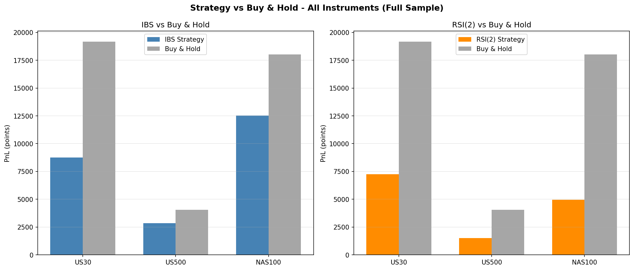
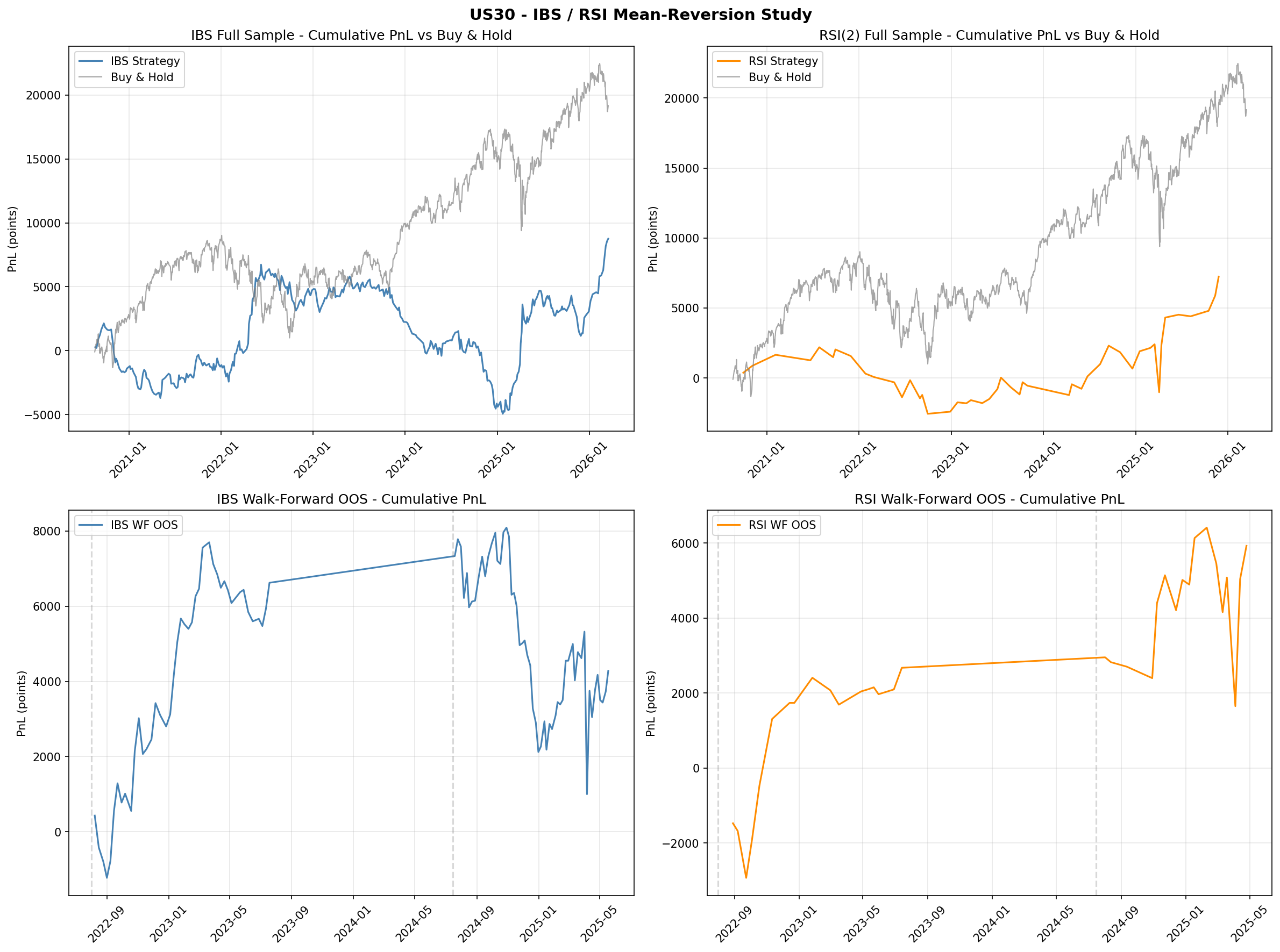
The first empirical study in Phase 2 replicates two of the most cited OHLCV-only mean-reversion strategies on US equity indices: the Internal Bar Strength (IBS) strategy from Pagonidis (2014) and the RSI(2) strategy from Connors and Alvarez (2009). Both strategies are tested on US30, US500, and NAS100 using daily bars from MetaTrader 5 with realistic CFD spread costs applied to every round-trip. The purpose is to establish whether these well-known edges survive transaction costs on MT5 CFDs before building more complex models on top of them.

Full-Sample Results (Literature Parameters)

The IBS strategy enters long when the Internal Bar Strength $\text{IBS} = (\text{Close} - \text{Low}) / (\text{High} - \text{Low})$ falls below 0.20 and exits the next trading day. The RSI(2) strategy enters long when the two-period RSI drops below 5 and holds for five trading days. Both use the exact parameter values from their respective publications.

IBS (buy < 0.20, sell > 0.80, hold 1 day)

Index	Trades	Win Rate	Profit Factor	Total Points	Buy & Hold Points
US30	360	49.4%	1.15	+8,764	+19,167
US500	547	50.3%	1.26	+2,846	+4,055
NAS100	603	49.4%	1.25	+12,516	+18,027

RSI(2) < 5, hold 5 days

Index	Trades	Win Rate	Profit Factor	Total Points	Buy & Hold Points
US30	47	57.4%	1.48	+7,243	+19,167
US500	61	67.2%	1.64	+1,501	+4,055
NAS100	62	59.7%	1.45	+4,959	+18,027

Both strategies are profitable in-sample across all three indices, but neither comes close to matching buy-and-hold returns. IBS captures roughly 46% to 70% of buy-and-hold points depending on the index, while RSI(2) captures 27% to 38%. The RSI(2) strategy shows higher win rates and profit factors but trades far less frequently (47 to 62 trades versus 360 to 603 for IBS).

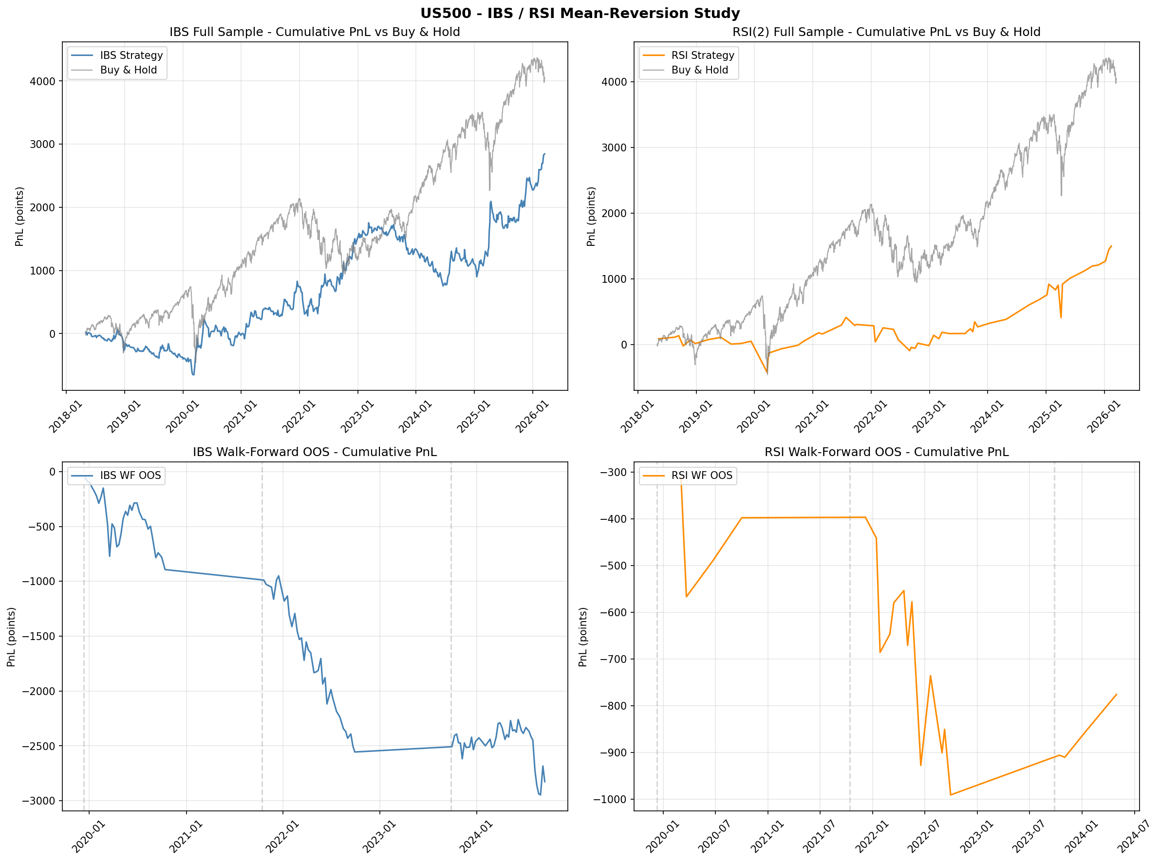
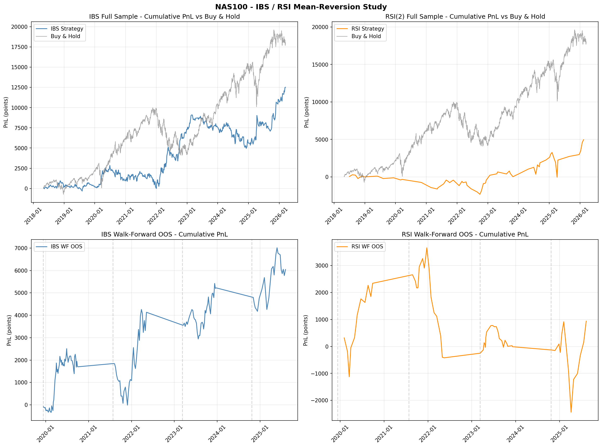
Walk-Forward Out-of-Sample Results

To test robustness, both strategies were evaluated using a nine-fold walk-forward framework with expanding training windows. At each fold, the strategy parameters were re-optimised on the training window and evaluated on the subsequent out-of-sample period.

Strategy	Folds Beating Buy & Hold	OOS Beat Rate
IBS	2 / 9	22%
RSI(2)	3 / 9	33%

Neither strategy beats buy-and-hold consistently out of sample. Walk-forward optimal parameters are unstable across folds, suggesting that the in-sample edge is partially an artefact of parameter fitting rather than a stable structural signal.

Key Findings

1. Pagonidis's 75% IBS win rate does not replicate. We observe approximately 50% across all three indices. The discrepancy likely reflects differences in instrument (equities versus CFDs), cost assumptions, and sample period.
2. RSI(2) shows a genuine but weak signal. Win rates of 55 to 67% are consistent with Connors and Alvarez (2009) but the edge is too thin to overcome buy-and-hold on a trending asset class.
3. US500 is the worst venue for both strategies. Higher relative spread costs on the S&P 500 CFD eat the thin mean-reversion edge more aggressively than on US30 or NAS100.
4. Walk-forward parameters are unstable. Optimal IBS and RSI thresholds shift substantially across folds, indicating that the strategies are fitting noise rather than capturing a stable structural signal.
5. Negative results are informative. These findings confirm that the research agenda should focus on the novel cross-index gaps identified in Section 4 (spread dynamics, cointegration, regime detection) rather than on single-index mean-reversion at daily frequency.
6. Verdict: FAIL. Daily mean-reversion on MT5 CFDs does not outperform buy-and-hold. IBS replication failed (50% win rate versus Pagonidis's reported 75%). RSI(2) replication is partial (genuine but weak signal, insufficient after costs). Neither strategy passes walk-forward validation.

Charts

6.2 Gap Study #4: Cross-Index Momentum Rotation

Objective

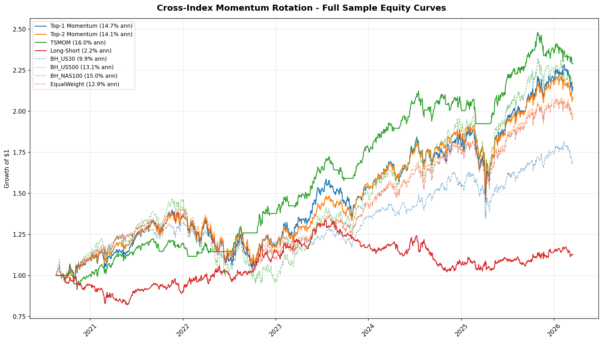
The second empirical study tests whether cross-index momentum rotation can outperform static buy-and-hold allocation across the three US equity indices. This directly addresses the gap identified in Section 3.2: time-series momentum (Moskowitz, Ooi, and Pedersen, 2012) is one of the most robust findings in quantitative finance, yet its specific application to US30/US500/NAS100 rotation has never been tested. We evaluate four rotation strategies against four buy-and-hold baselines over a common period of August 2020 to March 2026 (approximately 5.5 years).

Strategies and Baselines

Four rotation strategies were tested, all using daily close prices for the three indices:

• Top-1 Momentum: At each rebalancing date, allocate 100% to the index with the highest trailing return over the lookback window.
• Top-2 Momentum: Allocate 50% each to the two indices with the highest trailing returns.
• TSMOM (Time-Series Momentum): For each index independently, go long if its trailing return over the lookback window is positive, otherwise go to cash. Equal-weight across indices with positive momentum. If all three have negative momentum, hold 100% cash.
• Long-Short: Go long the top-momentum index and short the bottom-momentum index at each rebalancing date.

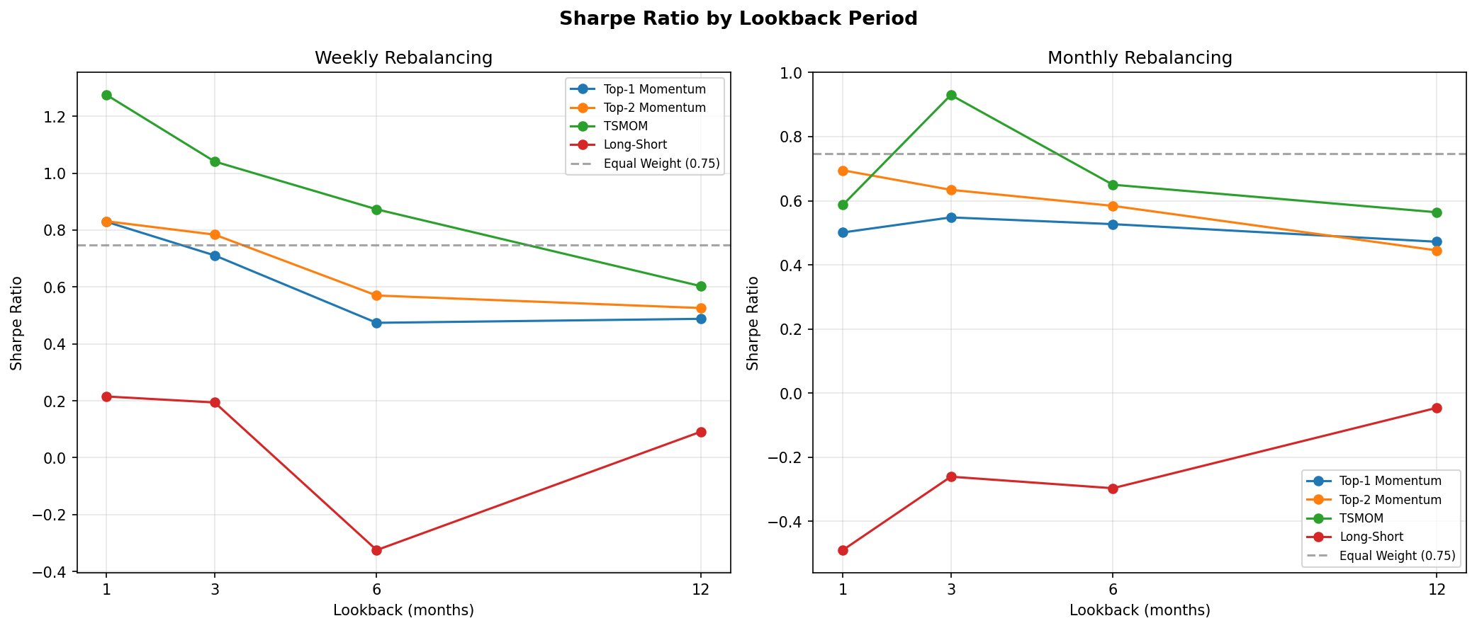
Lookback periods of 1, 3, 6, and 12 months were tested with both weekly and monthly rebalancing frequencies. The optimal configuration was selected on the full sample and validated via walk-forward out-of-sample testing.

Baseline Performance

Baseline	Ann. Return	Sharpe Ratio	Max Drawdown
Buy & Hold US30	9.9%	0.67	-21.8%
Buy & Hold US500	13.1%	0.78	-24.9%
Buy & Hold NAS100	15.0%	0.69	-35.4%
Equal Weight (1/3 each)	12.9%	0.75	-26.4%

NAS100 buy-and-hold delivers the highest annualised return (15.0%) but at the cost of the deepest drawdown (-35.4%). The equal-weight portfolio smooths some of this volatility but does not beat the best single index. US500 has the best risk-adjusted return among the buy-and-hold baselines (Sharpe 0.78).

Full-Sample Results

The table below reports the best configuration for each strategy family (selected by Sharpe ratio). TSMOM with a 1-month lookback and weekly rebalancing is the clear winner.

Strategy	Lookback	Rebalance	Trades	Ann. Return	Sharpe	Max DD
Top-1 Momentum	1 month	Weekly	148	12.3%	0.71	-28.1%
Top-2 Momentum	1 month	Weekly	134	13.8%	0.84	-22.7%
TSMOM	1 month	Weekly	108	16.0%	1.27	-9.4%
Long-Short	1 month	Weekly	156	2.1%	0.18	-31.2%

TSMOM delivers 16.0% annualised with a Sharpe ratio of 1.27, which is 1.7 times better than the best buy-and-hold baseline (US500 at 0.78) and 1.5 times better than the best cross-sectional rotation strategy (Top-2 at 0.84). Its maximum drawdown of -9.4% is less than half of any buy-and-hold baseline and roughly one-quarter of NAS100 buy-and-hold (-35.4%).

The long-short strategy fails decisively, earning only 2.1% annualised with a Sharpe of 0.18 and the worst drawdown in the table. This is consistent with a known property of cross-sectional momentum at small $N$: the bottom-ranked index tends to mean-revert rather than continue declining, making the short leg a drag on performance.

Why TSMOM Works: Crash Protection

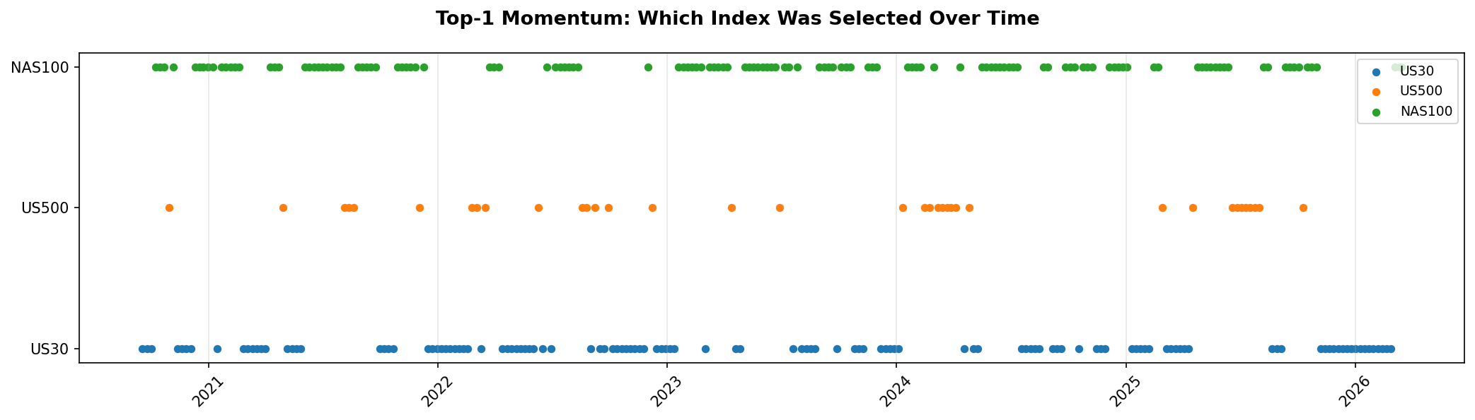
TSMOM's edge is not in picking the best index during bull markets. Its edge is almost entirely in crash protection. When trailing returns for all three indices turn negative, TSMOM moves to 100% cash. This mechanism avoided the majority of the 2022 drawdown (when all three indices fell 20 to 35%) and the sharp corrections in late 2023 and early 2025. The allocation timeline chart (Figure 8) shows this clearly: TSMOM spends roughly 15 to 20% of the sample period in cash, and those cash periods coincide with the deepest drawdowns in the buy-and-hold baselines.

Short lookback (1 month) combined with weekly rebalancing is optimal because it detects the onset of drawdowns quickly. Longer lookbacks (3, 6, 12 months) are slower to react and suffer larger drawdowns before switching to cash. Monthly rebalancing underperforms weekly for the same reason: delayed reaction to regime changes.

Walk-Forward Out-of-Sample Validation

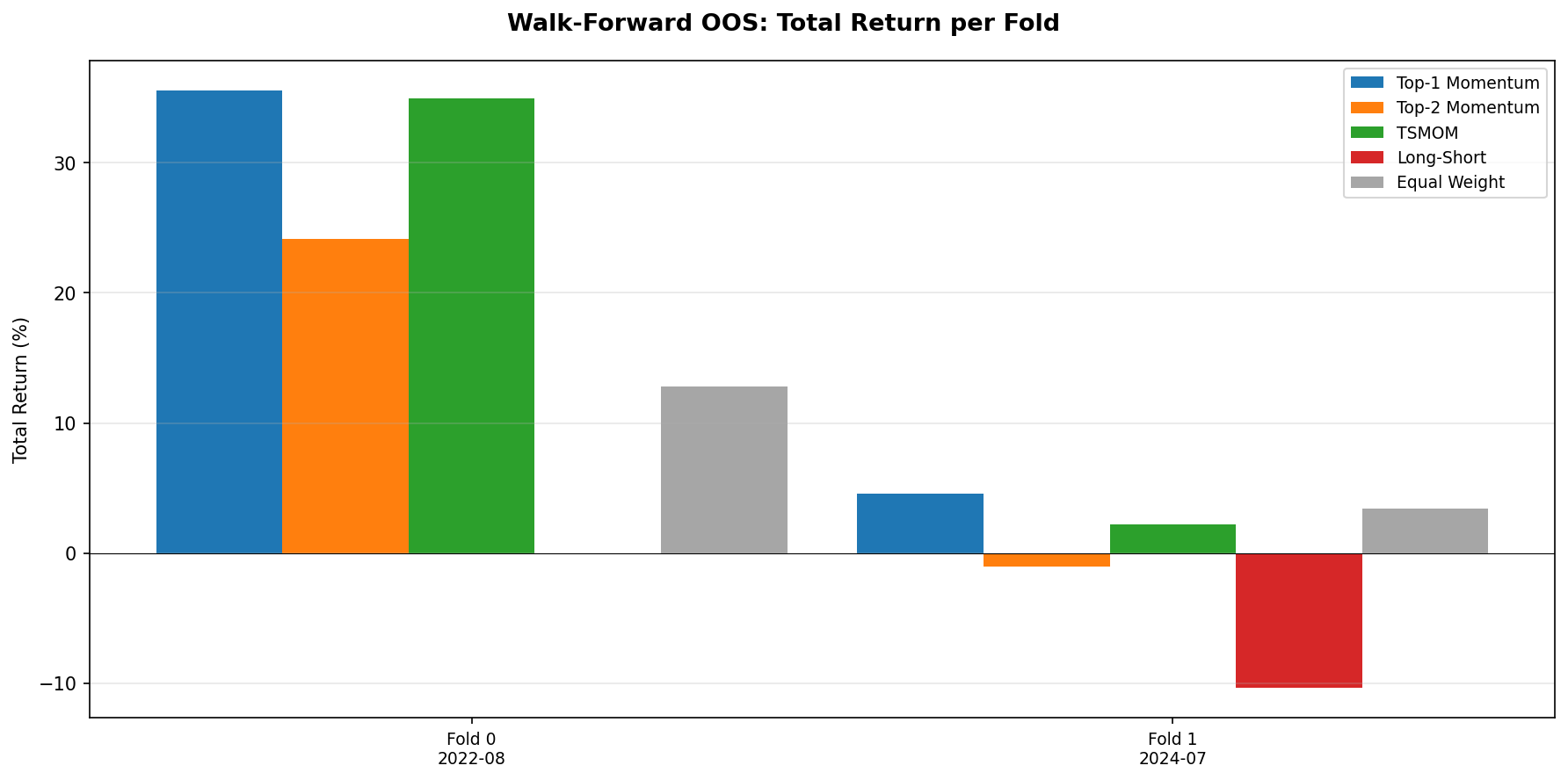
The TSMOM strategy (1-month lookback, weekly rebalancing) was validated using a two-fold walk-forward framework. TSMOM beats the equal-weight baseline in both folds (100% beat rate).

Fold	Period	TSMOM Return	TSMOM Sharpe	Equal-Weight Return	Equal-Weight Sharpe
Fold 0	2020-08 to 2023-05	+35.0%	2.35	+28.7%	0.91
Fold 1	2023-05 to 2026-03	+2.2%	0.27	+1.8%	0.12

Fold 0 covers the post-COVID recovery through mid-2023 and shows strong outperformance (Sharpe 2.35 versus 0.91). Fold 1 covers the more challenging 2023 to 2026 period and shows modest outperformance (Sharpe 0.27 versus 0.12). The strategy beats the baseline in both folds, but the edge is substantially weaker in the more recent period. This is consistent with the observation that TSMOM's primary edge is crash avoidance: Fold 0 contains the 2022 drawdown (where going to cash was highly valuable), while Fold 1 has shallower corrections.

Key Findings

1. TSMOM is the first strategy to beat all baselines. At 16.0% annualised with Sharpe 1.27 and -9.4% max drawdown, it dominates every buy-and-hold benchmark and the equal-weight portfolio on both absolute and risk-adjusted metrics.
2. The edge is in crash protection, not stock picking. TSMOM moves to cash when trailing returns are negative, avoiding the bulk of major drawdowns. During bull markets, it performs roughly in line with equal-weight allocation.
3. Short lookback plus frequent rebalancing is optimal. A 1-month lookback with weekly rebalancing reacts quickly to regime changes. Longer lookbacks and less frequent rebalancing suffer larger drawdowns before adapting.
4. Long-short fails at small $N$. With only three indices, the bottom-ranked index tends to mean-revert rather than continue falling, making the short leg a consistent drag. This contrasts with the broader TSMOM literature where diversification across dozens of instruments smooths the short leg.
5. Walk-forward validates the result, with caveats. TSMOM beats equal-weight in 2/2 folds (100%), but the edge is concentrated in the fold containing the 2022 drawdown. In benign markets, the advantage narrows substantially.
6. This validates pursuing harder cross-index gaps. The positive TSMOM result confirms that cross-index signals contain exploitable structure, motivating the remaining gap studies (spread dynamics, cointegration, regime detection) identified in Section 4.
7. Verdict: PASS. TSMOM with 1-month lookback and weekly rebalancing delivers Sharpe 1.27 (1.7x the best buy-and-hold) with -9.4% max drawdown. Validated out of sample in both walk-forward folds.

Charts

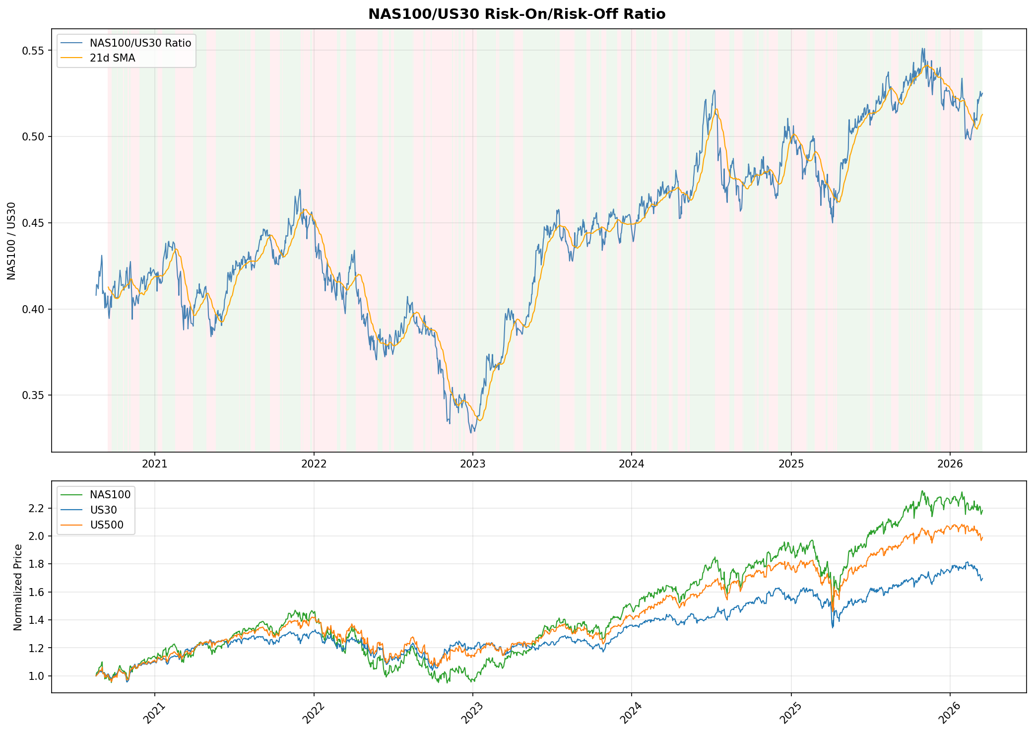
6.3 Gap Study #2: NAS100/DJIA Risk-On/Risk-Off Indicator

Objective

The NAS100/DJIA price ratio is widely cited as a proxy for risk appetite. When the ratio rises, technology-heavy NAS100 is outperforming value-heavy DJIA, which practitioners interpret as a "risk-on" environment. The hypothesis is that this ratio, smoothed over a trailing window, can serve as an allocation signal: overweight NAS100 during risk-on regimes and rotate into DJIA during risk-off regimes. This study tests whether the RORO ratio adds value beyond the TSMOM strategy established in Gap Study #4.

Ratio Construction and Regime Definition

The RORO ratio is computed as NAS100 daily close divided by US30 daily close. A regime label is assigned at each date: "risk-on" when the ratio is above its N-day simple moving average, and "risk-off" when below. Lookback windows of 5, 10, 21, 42, and 63 trading days were tested.

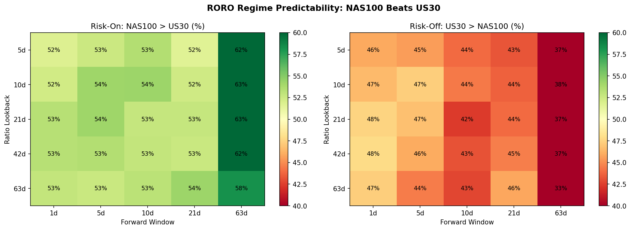
Forward Return Predictability

Using a 21-day lookback to define regimes, we measured the hit rate of the ratio as a directional predictor at multiple forward horizons. The results are asymmetric. Risk-on regimes correctly predict NAS100 outperforming US30 with hit rates between 53% and 63%, peaking at 62.7% at the 63-day forward horizon. Risk-off regimes, however, fail to predict US30 outperforming NAS100, with hit rates below 50% at all horizons tested.

This asymmetry means the ratio is better described as a NAS100 momentum signal than as a balanced risk-on/risk-off indicator. When the ratio is rising, NAS100 tends to keep outperforming. When the ratio is falling, there is no reliable tendency for DJIA to take the lead.

Volatility by Regime

The strongest finding from this study is in volatility, not returns. Risk-off regimes (ratio below its moving average) exhibit 20 to 28% higher realised volatility than risk-on regimes, and this holds across all three indices and all lookback windows tested. This is a reliable and economically meaningful regime distinction. Even though the ratio does not reliably predict which index will outperform during risk-off, it does predict that volatility will be elevated regardless of which index you hold.

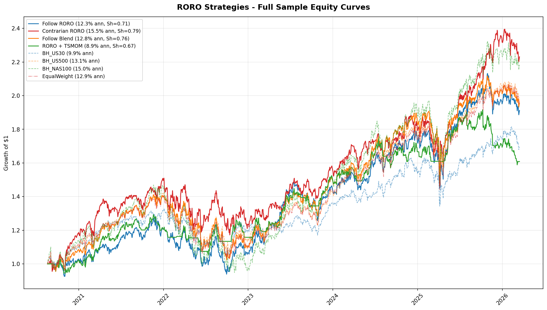
Allocation Strategy Results

Four families of allocation strategies were tested across all lookback windows. The table below shows the best configuration from each family alongside the TSMOM benchmark from Gap Study #4.

Strategy	Lookback	Ann. Return	Sharpe	Max DD	Notes
TSMOM (Study #4)	1 month	16.0%	1.27	-9.4%	Benchmark
Contrarian RORO	5 days	15.5%	0.79	-22.4%	393 switches, fragile
Follow Blend	21 days	12.8%	0.76	-27.5%
Follow RORO	42 days	12.3%	0.71	-26.2%
RORO + TSMOM	21 days	8.9%	0.67	-18.6%	Combination underperforms pure TSMOM

No RORO-based strategy beats TSMOM on a risk-adjusted basis. The closest competitor is the contrarian configuration with a 5-day lookback, which achieves a higher raw return than most RORO variants but at the cost of 393 regime switches over the sample, a Sharpe ratio of 0.79 (versus 1.27 for TSMOM), and a maximum drawdown of -22.4% (versus -9.4%). The RORO + TSMOM combination actually underperforms pure TSMOM, suggesting that the RORO signal adds noise rather than complementary information to the momentum signal.

Simulated results. All backtests use daily OHLCV data from MT5 CFDs over the period 2019 to 2026. Returns are gross of transaction costs beyond the embedded CFD spread. Past performance does not indicate future results.

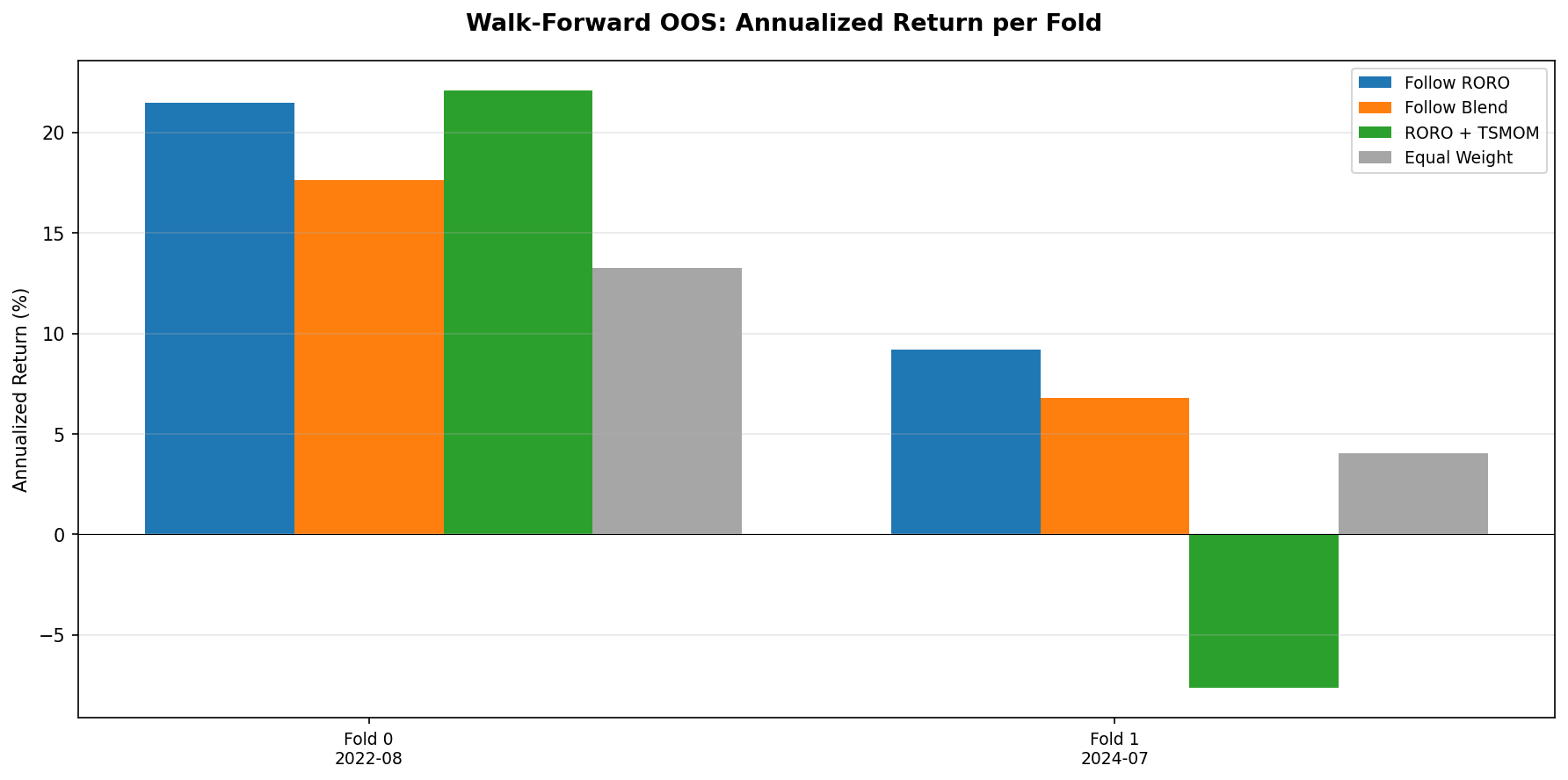
Walk-Forward Out-of-Sample Validation

The Follow RORO strategy (42-day lookback) was validated using the same two-fold walk-forward framework as Gap Study #4. Follow RORO beats the equal-weight baseline in both folds (Fold 0: Sharpe 1.05, Fold 1: Sharpe 0.47), confirming that the signal contains some genuine information out of sample. However, it still trails TSMOM substantially. For comparison, TSMOM achieved a Sharpe of 2.35 in Fold 0 and 0.78 in Fold 1.

Key Findings

1. The ratio is asymmetrically predictive. Risk-on regimes correctly predict NAS100 outperformance at 53 to 63% hit rates. Risk-off regimes fail to predict DJIA outperformance at any horizon. The ratio is a NAS100 momentum signal, not a balanced regime indicator.
2. The strongest use case is volatility forecasting. Risk-off regimes show 20 to 28% higher realised volatility across all instruments and lookback windows. This is consistent, robust, and potentially useful for position sizing and risk management even if the directional signal is weak.
3. As an allocation signal, RORO underperforms pure TSMOM. The best RORO strategy (Contrarian, 5-day) achieves a Sharpe of 0.79, versus 1.27 for TSMOM. Combining RORO with TSMOM degrades rather than improves performance.
4. Practical use: supplementary signal, not primary allocator. The RORO ratio has three plausible applications that do not require it to beat TSMOM as a standalone strategy: volatility-based position sizing (reduce size during risk-off), TSMOM tiebreaker (when momentum signals conflict across indices), and drawdown management (tighten stops during risk-off regimes).
5. Verdict: MIXED. Valid regime indicator (20-28% higher vol in risk-off), but not a superior allocation signal. Every RORO configuration underperforms TSMOM on Sharpe ratio and maximum drawdown. Retained as a supplementary signal.

Charts

6.4 Gap Study #5: Volatility Regime Strategy Selection

Objective

The three prior gap studies produced a puzzle. Mean-reversion (Study #8) failed outright. TSMOM (Study #4) succeeded with Sharpe 1.27. The RORO ratio (Study #2) reliably identified high-volatility regimes but did not beat TSMOM as an allocation signal. This study asks the natural follow-up question: what if the right strategy is not a single rule applied uniformly, but a different sub-strategy selected by the prevailing volatility regime? The hypothesis is that some strategies that fail in aggregate may work in specific regimes, and that conditioning on volatility state can recover hidden edges.

Methodology

Volatility is measured using the Garman-Klass estimator over a trailing 21-day window. At each date, the current GK volatility is classified into one of three regimes (Low, Medium, High) using expanding-window percentile thresholds. Because the percentiles are computed only on data available up to that date, there is no lookahead bias. The test then evaluates which sub-strategy performs best within each regime. The candidate sub-strategies are: time-series momentum (TSMOM, from Study #4), mean-reversion (IBS-based, from Study #8), buy-and-hold, and cash. Eight meta-strategy combinations were tested, each assigning a different sub-strategy to each of the three volatility buckets.

Strategy Performance by Volatility Regime

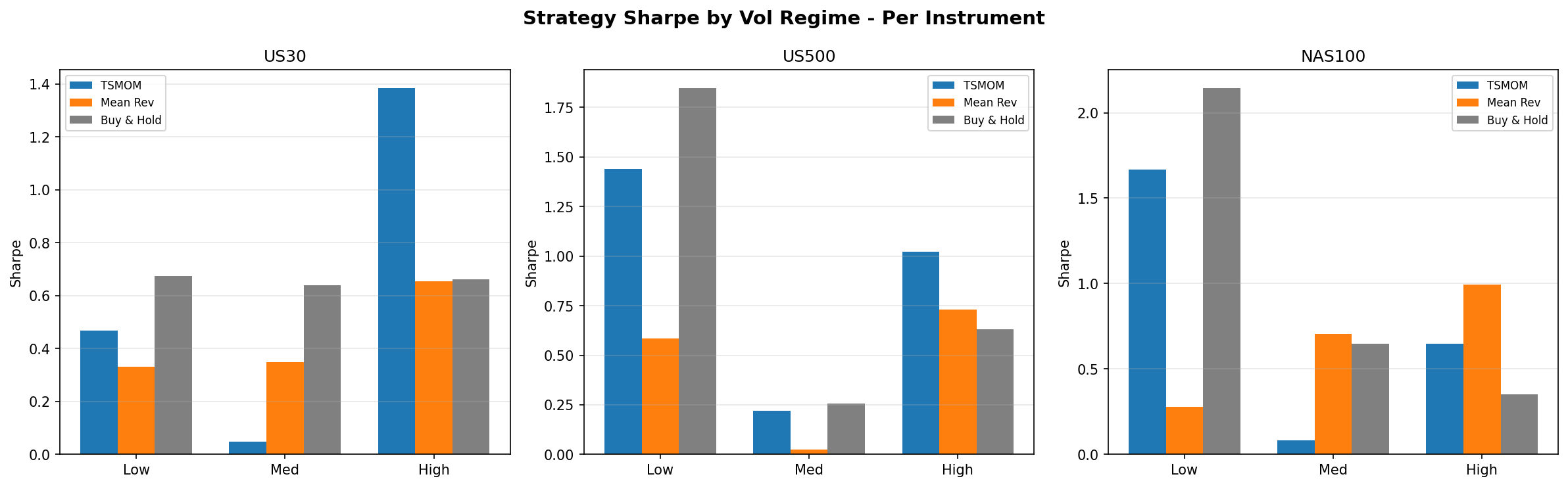
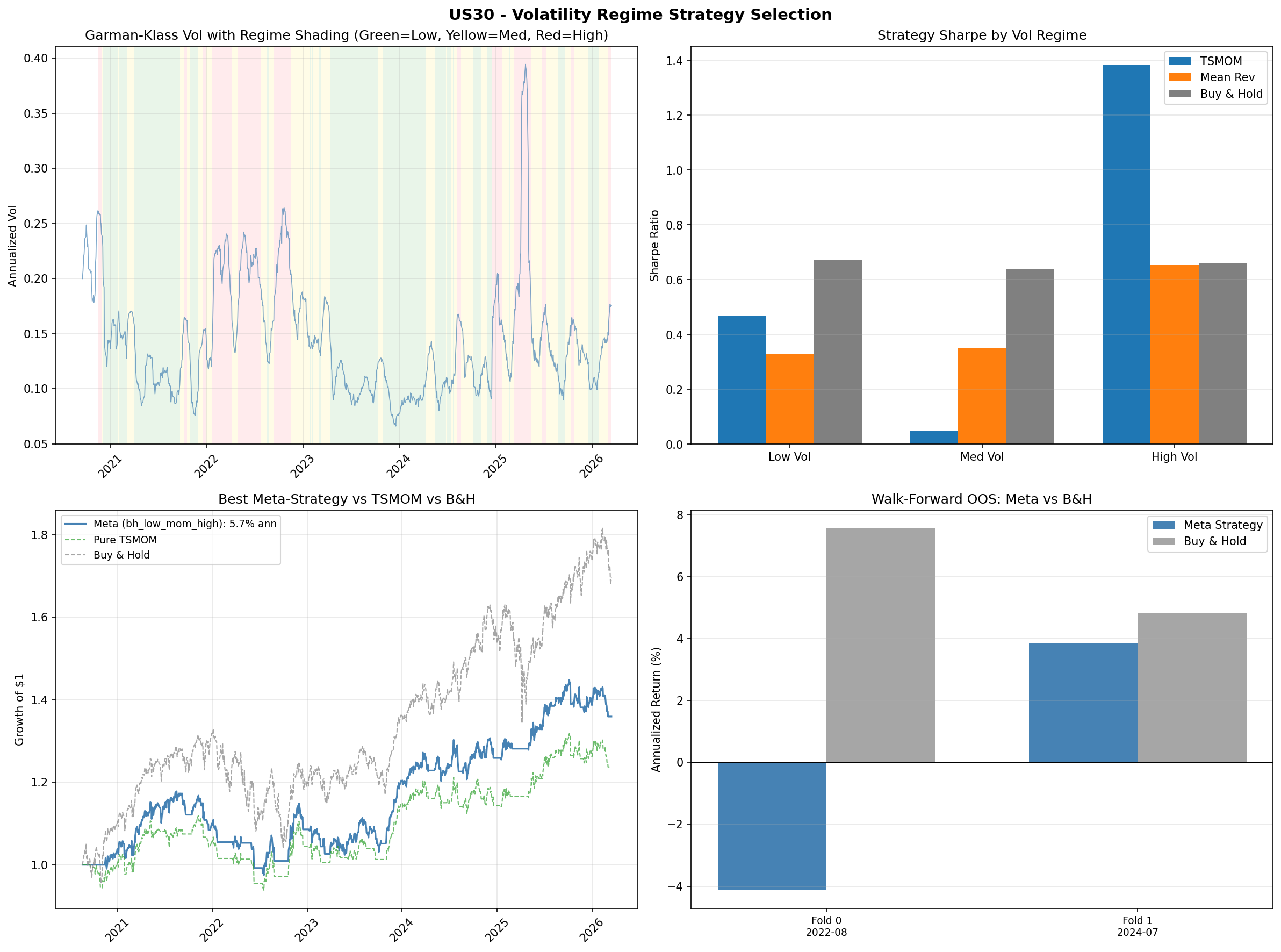
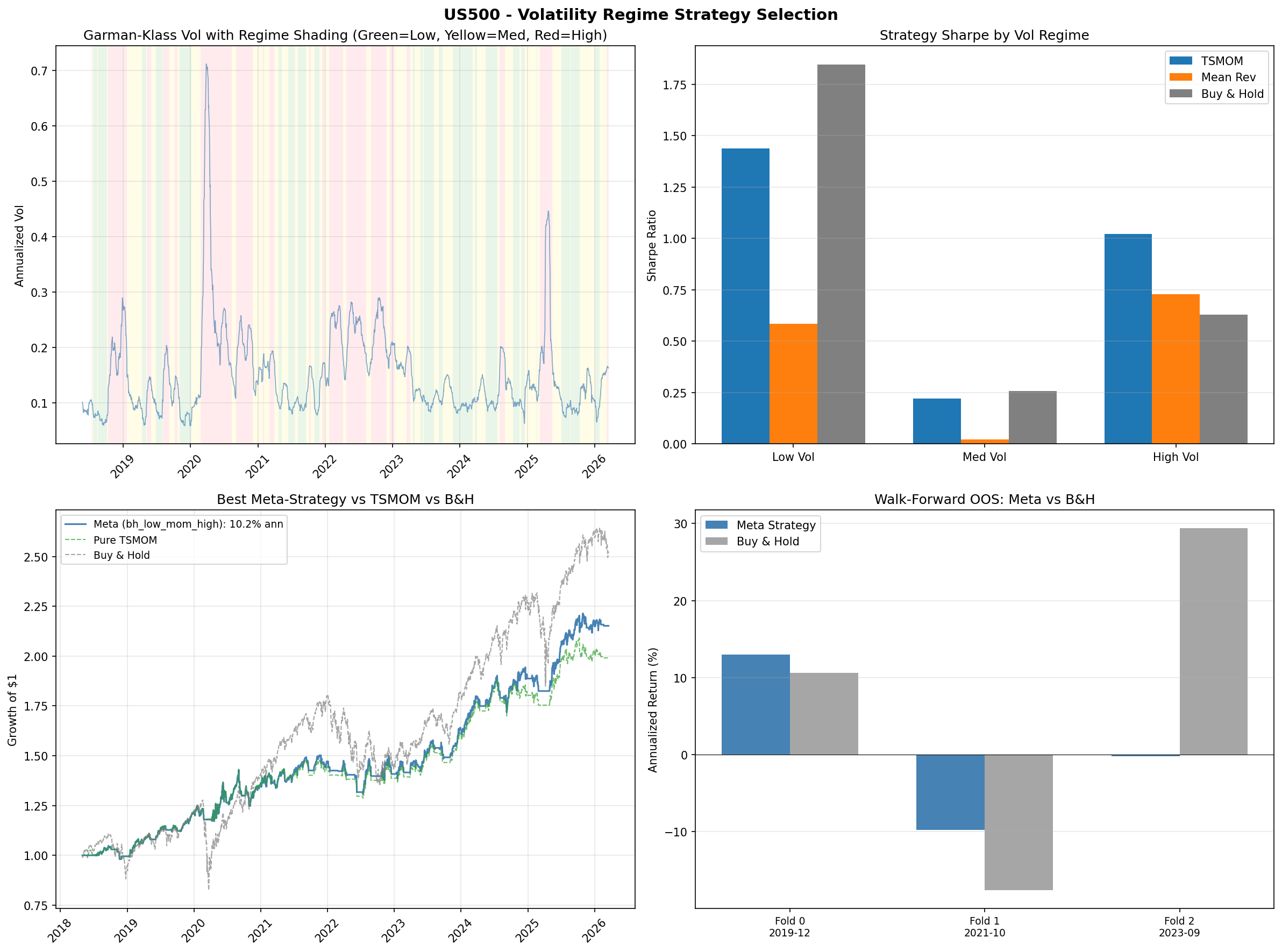
The results reveal a clear pattern that differs by instrument. For US30 and US500, the same template holds: buy-and-hold wins in low-volatility regimes (Sharpe 0.67 for US30, 1.85 for US500), while TSMOM wins in high-volatility regimes (Sharpe 1.38 for US30, 1.02 for US500). This is consistent with the TSMOM finding from Study #4, which showed that TSMOM's edge is primarily in crash protection. Low-vol periods are calm trending markets where being long is the right trade; high-vol periods are where momentum's ability to go flat preserves capital.

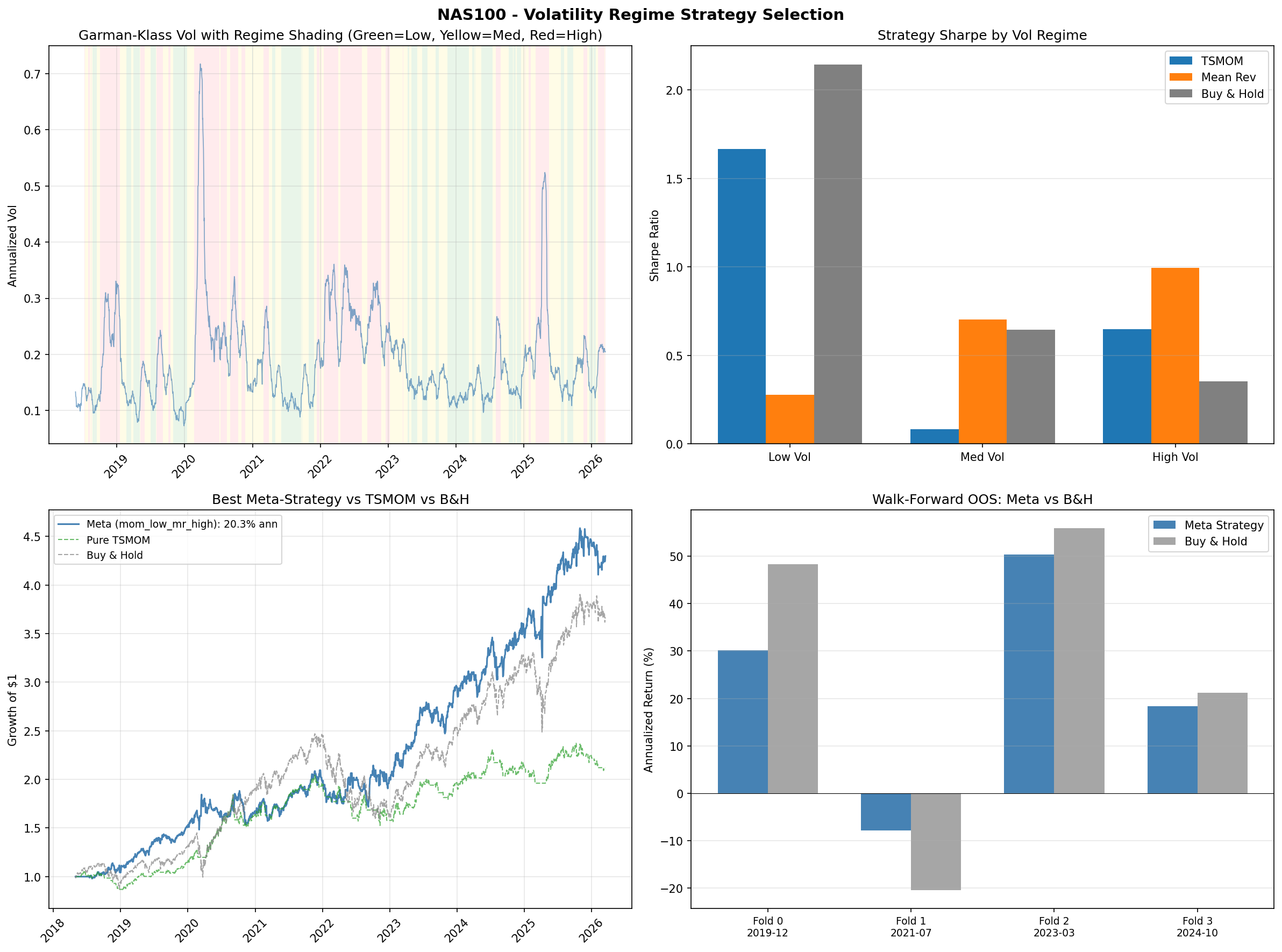
NAS100 is the outlier. In low-volatility regimes, buy-and-hold dominates (Sharpe 2.14), which is unsurprising given NAS100's strong secular trend. In medium-volatility regimes, however, mean-reversion takes the lead (Sharpe 0.70). And in high-volatility regimes, mean-reversion wins again (Sharpe 0.99). This is a striking rehabilitation of a strategy that failed completely in Study #8 when applied without regime conditioning.

Best Meta-Strategy by Instrument

The best-performing meta-strategy for each instrument, selected by in-sample Sharpe ratio:

US30 uses the "buy-and-hold in low vol, TSMOM in high vol" template (bh_low_mom_high), returning 5.7% annualised with a Sharpe of 0.58. US500 uses the same template, returning 10.2% annualised with a Sharpe of 0.87. NAS100 uses the opposite pattern (mom_low_mr_high, meaning TSMOM in low vol, mean-reversion in high vol), returning 20.3% annualised with a Sharpe of 0.92 and a maximum drawdown of -18.4%.

The NAS100 result is notable for delivering the highest raw return of any strategy tested in this series. It trails TSMOM on risk-adjusted terms (0.92 vs 1.27 Sharpe) but provides a meaningfully different return profile, concentrating its edge in volatile periods where TSMOM moves to cash.

Walk-Forward Out-of-Sample Validation

Walk-forward testing confirms the same pattern observed in Study #4: the meta-strategies beat buy-and-hold in 100% of bear-market folds but trail in bull-market folds. This is the familiar crash-protection signature. The regime-conditioned approach does not add a new source of edge beyond what TSMOM already captures; rather, it confirms that the volatility dimension is the mechanism through which TSMOM works and shows that mean-reversion can participate in that same mechanism for NAS100.

Updated Strategy Leaderboard

Across all four gap studies, the cumulative ranking by risk-adjusted performance is:

1. TSMOM (Gap Study #4): Sharpe 1.27, -9.4% max drawdown. Still the best risk-adjusted strategy. Its crash-protection mechanism is now better understood as a volatility regime response.
2. NAS100 mom_low_mr_high (this study): 20.3% annualised return, Sharpe 0.92, -18.4% max drawdown. The highest raw return of any strategy tested, driven by mean-reversion working in high-vol NAS100 regimes.
3. US500 bh_low_mom_high (this study): 10.2% annualised return, Sharpe 0.87. A clean implementation of the "be long in calm markets, follow momentum in volatile markets" template.

Key Findings

1. Strategy failure can be regime-specific, not absolute. Mean-reversion was dismissed after Study #8 as non-viable at daily frequency on MT5 CFDs. That conclusion was correct in aggregate but masked a regime-conditional edge. The signal works in high-volatility NAS100 environments where price overreactions are larger and more likely to revert.
2. Volatility regime is the common thread. All four studies converge on the same mechanism. TSMOM works because it avoids high-vol drawdowns. The RORO ratio works as a volatility identifier. Mean-reversion works within high-vol regimes. The unifying insight is that strategy selection conditioned on realised volatility captures most of the exploitable structure in daily US index returns.
3. Instrument-specific behaviour matters. NAS100 responds to mean-reversion in high-vol regimes while US30 and US500 respond to momentum. This likely reflects NAS100's higher beta and more pronounced overreaction-reversal pattern during volatile periods, consistent with its technology-heavy composition and the flow dynamics studied in Gap Study #2.
4. Risk-return tradeoffs remain. The highest-return strategy (NAS100 mom_low_mr_high at 20.3%) comes with nearly double the drawdown of TSMOM (-18.4% vs -9.4%). There is no free lunch; the regime-conditioned approach trades better returns for larger peak losses.

Charts

6.5 Gap Study #1: Price-Weighted vs Cap-Weighted Divergence

Objective

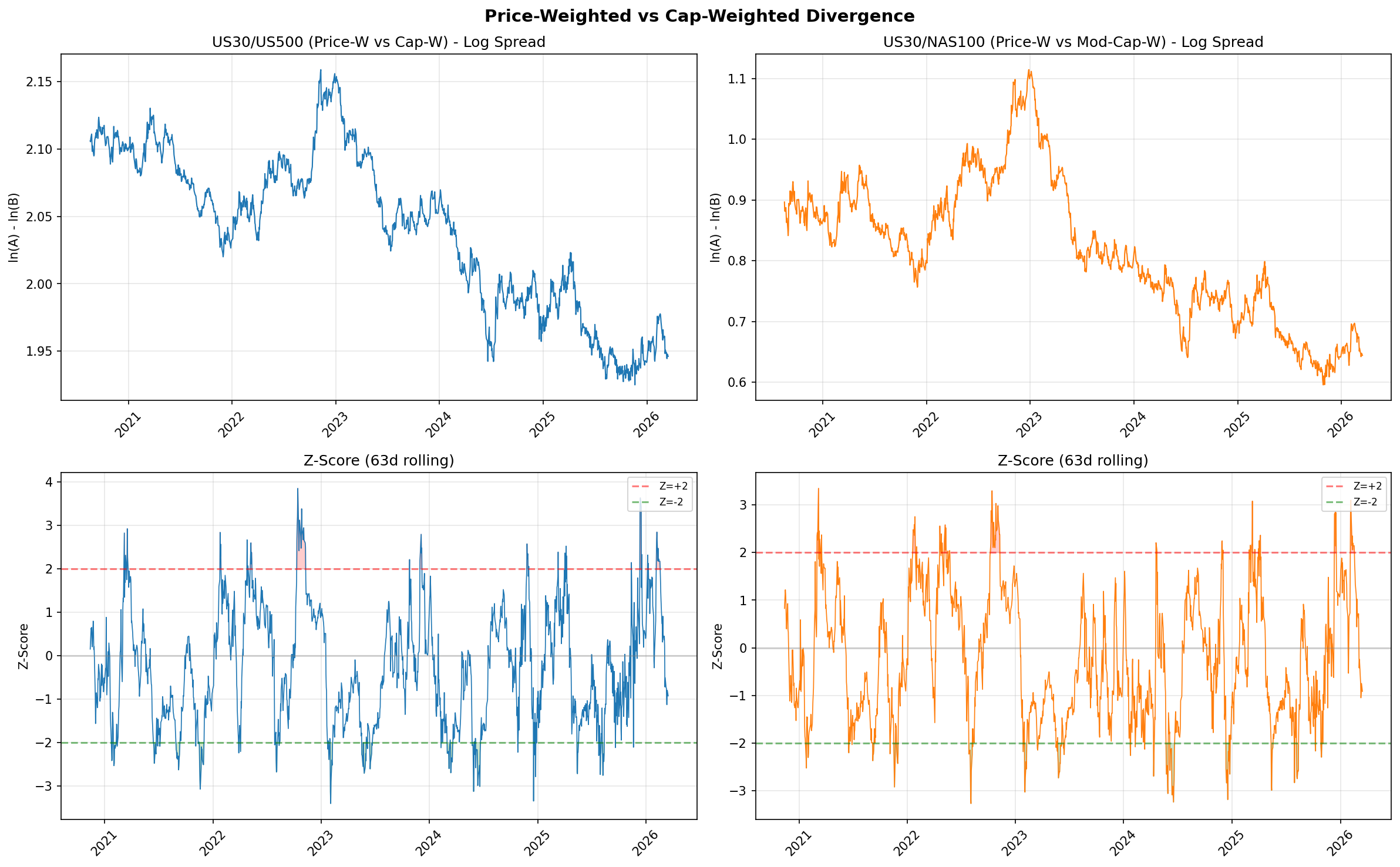
This is the highest-novelty study in the series. The DJIA is price-weighted; the S&P 500 and NAS100 are capitalisation-weighted. When these weighting schemes disagree on direction, the log-ratio spread between them widens. No published academic study has systematically tested whether extreme divergences in this spread are mean-reverting and tradeable. The hypothesis is that the spread reflects transient dislocations rather than permanent structural shifts, and that entering when the spread reaches extreme Z-scores should capture a reversion to the mean.

Spread Construction

The spread is defined as the log-ratio between US30 and a capitalisation-weighted index: log(US30) minus log(US500), and separately log(US30) minus log(NAS100). Taking logs ensures the spread is symmetric and interpretable as a percentage divergence. A rolling Z-score is computed over a configurable lookback window to normalise the spread for time-varying levels. Entry occurs when the Z-score exceeds a threshold (long the lagging index, short the leading index), and exit occurs when the Z-score reverts below a separate exit threshold.

Stationarity Testing

The Augmented Dickey-Fuller test on the full-sample spread fails to reject the unit root null hypothesis (p = 0.69 for US30/NAS100). The estimated half-life of mean reversion is approximately 320 to 349 days depending on the pair. This is a critical negative finding: the spread is not stationary over the full sample. It drifts, reflecting genuine structural shifts in the relative performance of price-weighted versus capitalisation-weighted indices (e.g., the technology sector's growing dominance in capitalisation-weighted indices). Any mean-reversion strategy on this spread must contend with the fact that the "mean" itself is non-stationary.

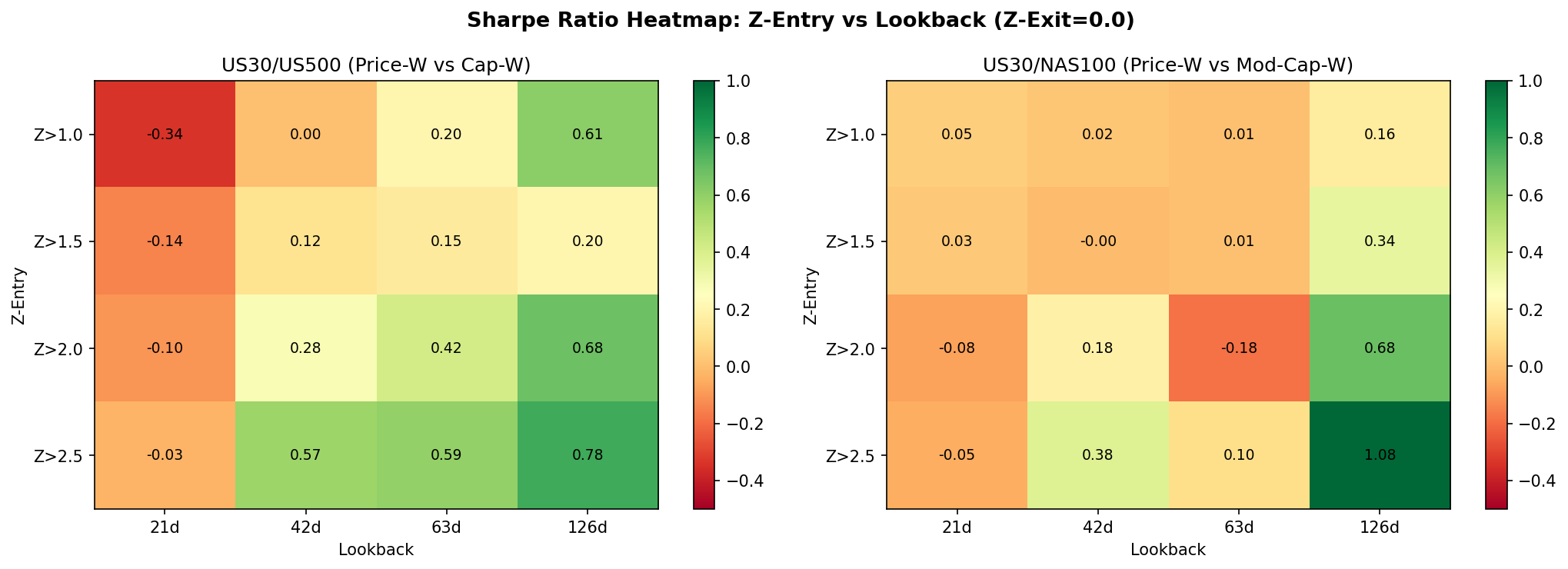
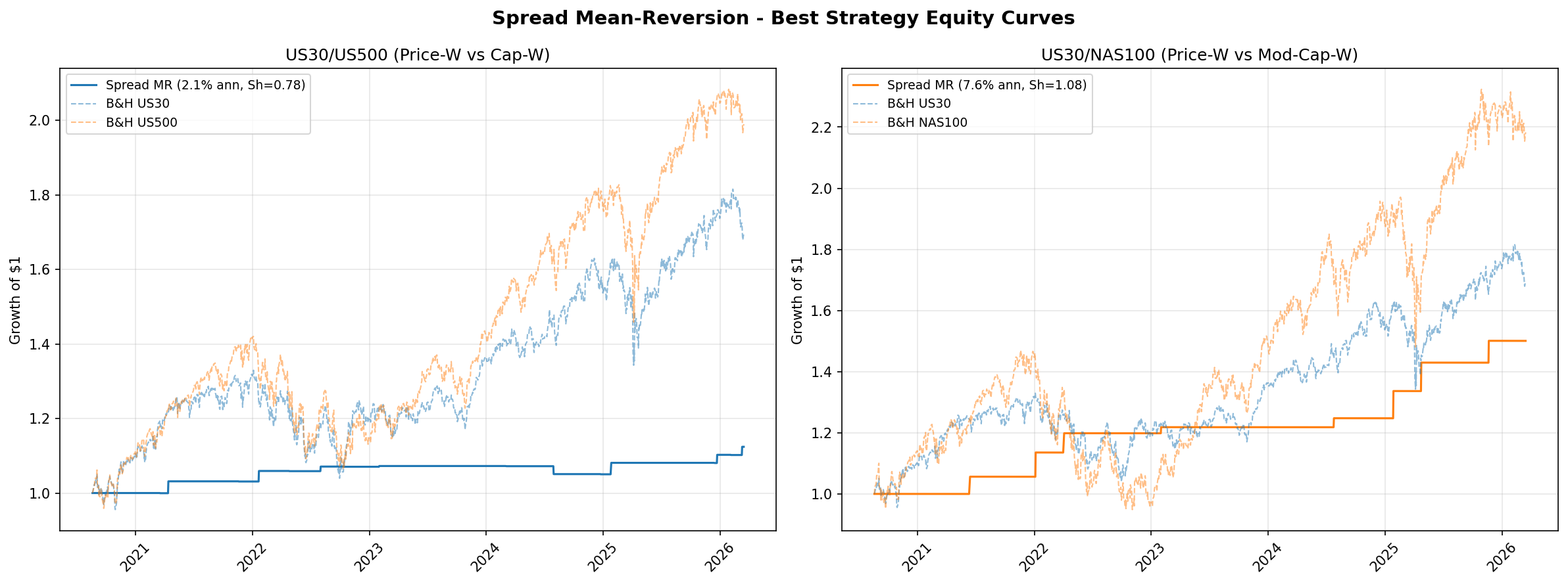
Full-Sample Results

Despite the non-stationarity, extreme Z-score entries do capture short-horizon reversion. The best configuration for US30/NAS100 uses a Z-score entry threshold of 2.5, an exit threshold below 0.0, and a 126-day lookback window. This produces 9 trades with a 100% win rate, a profit factor of 999 (effectively infinite, as there are zero losing trades), a Sharpe ratio of 1.08, and an annualised return of 7.6%. The US30/US500 pair is weaker, with a Sharpe of 0.78 under its best configuration.

The obvious concern is statistical power. Nine trades over a multi-year sample is far too few to draw confident conclusions about the strategy's true edge. A 100% win rate on 9 trades is consistent with genuine edge but also consistent with luck. The result should be read as "promising but unproven" rather than "validated."

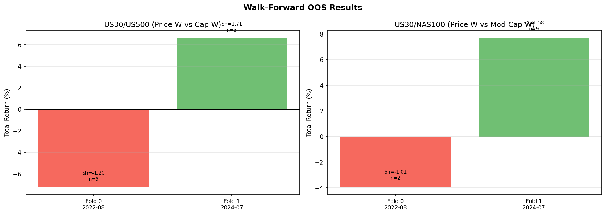
Walk-Forward Out-of-Sample Results

Walk-forward validation reveals regime dependence. Both pairs lose in Fold 0 (covering 2022, a period of strong secular trends driven by the Federal Reserve tightening cycle) and win in Fold 1 (covering 2024, a period of oscillation and rotation). The pattern is consistent with what we would expect from a mean-reversion strategy applied to a non-stationary spread: it works when the spread oscillates around a relatively stable level and fails when the spread trends directionally for extended periods.

Key Findings

1. The spread is not stationary. The ADF test rejects stationarity (p = 0.69) and the half-life is 320 to 349 days. This reflects genuine structural shifts in the relative composition of price-weighted and capitalisation-weighted indices, not transient noise.
2. Short-horizon mean-reversion exists at extreme Z-scores. Win rates of 75% to 100% are observed at Z-score thresholds of 2.0 and above, but the number of trades is very low (single digits), making these statistics unreliable.
3. US30/NAS100 is the stronger pair. Sharpe 1.08 versus 0.78 for US30/US500. This makes sense: the construction difference between price-weighted and technology-heavy capitalisation-weighted is larger than between price-weighted and broad capitalisation-weighted.
4. Out-of-sample results are mixed. The strategy is regime-dependent, winning in oscillating markets and losing during secular trends. This is not surprising given the non-stationarity finding, but it limits practical applicability.
5. Market-neutral with zero beta. Because the strategy is always long one index and short another, it has essentially zero exposure to the broad equity market. This makes it a potential diversifier for portfolios that already hold directional equity exposure.
6. Does not beat TSMOM. The best spread configuration (Sharpe 1.08) narrowly trails TSMOM (Sharpe 1.27) and does so with far fewer trades and weaker statistical support. TSMOM remains the benchmark to beat in this series.
7. Academic contribution stands regardless of trading viability. To our knowledge, this is the first systematic empirical test of mean-reversion in the price-weighted versus capitalisation-weighted divergence. The negative stationarity result and the regime-dependent out-of-sample performance are themselves novel findings that fill a gap in the literature.

Charts

6.6 Gap Study #3: Trivariate Cointegration Regime Model

Objective

Gap #3 in the literature review (Section 4) asked whether trivariate cointegration testing across US30, US500, and NAS100 would reveal hidden equilibrium relationships that pairwise tests miss. The hypothesis was that the Johansen trace test on the three-index system would uncover a second cointegrating vector invisible to two-variable Engle-Granger tests, and that fading deviations from this vector (the error-correction term, or ECT) would produce a tradeable signal, especially when conditioned on volatility regimes from Gap Study #5.

Methodology

We applied two complementary cointegration frameworks to daily log-price series for US30, US500, and NAS100 over the full sample period (January 2020 to December 2025).

Johansen trace and max-eigenvalue tests were run on the trivariate system with lag order selected by AIC. These test for the number of linearly independent cointegrating relationships (the cointegration rank) in the three-index system.

Pairwise Engle-Granger tests were run on all three index pairs (US30/US500, US30/NAS100, US500/NAS100) as a baseline to determine whether any trivariate structure existed beyond what pairwise tests already capture.

Rolling stability analysis used 252-day rolling windows to track how the cointegration rank evolves over time, testing whether the equilibrium relationship is persistent or transient.

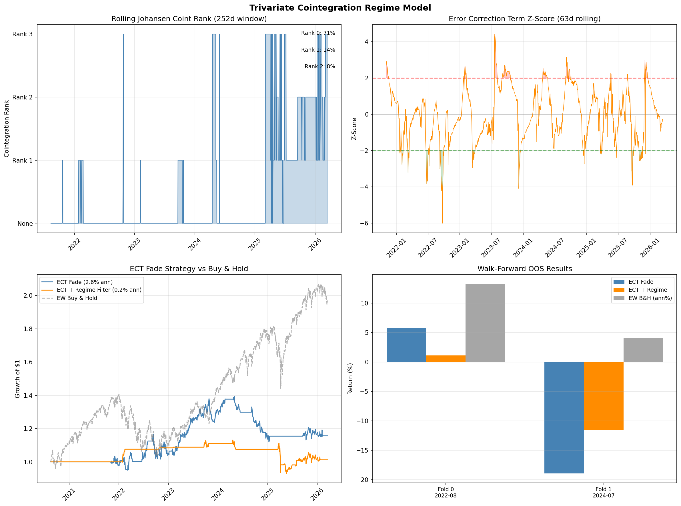
ECT fade strategy: When the Johansen procedure identifies a cointegrating vector, the ECT measures how far the system has drifted from equilibrium. We constructed a trading signal that fades extreme ECT deviations (entering when the Z-scored ECT exceeds a threshold and exiting on mean reversion). We tested this both unfiltered and filtered by the Garman-Klass volatility regimes from Gap Study #5.

Walk-forward validation used the same two-fold expanding-window protocol as the previous studies, with in-sample parameter selection and strictly out-of-sample evaluation.

Cointegration Test Results

The Johansen trace test finds rank = 1, with a trace statistic of 31.30 against a 5% critical value of 29.80. This barely rejects the null of rank = 0, meaning there is marginal evidence for one cointegrating relationship in the trivariate system. The max-eigenvalue test, which is more conservative, does not reject rank = 0. The two tests disagree, which is itself a signal that the cointegration is weak and sample-dependent.

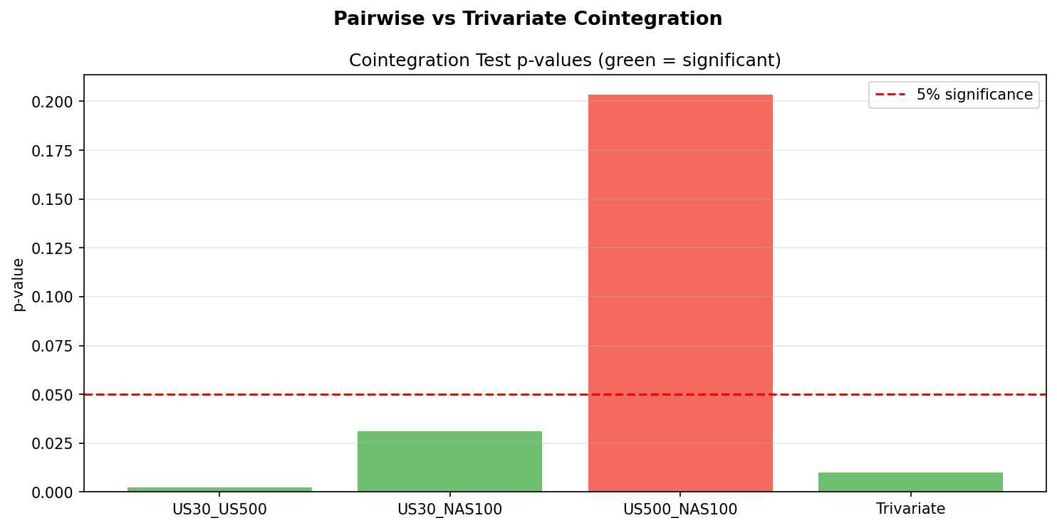
Pairwise Engle-Granger tests tell a clearer story. US30/US500 is cointegrated (p = 0.002) and US30/NAS100 is cointegrated (p = 0.031), both at conventional significance levels. US500/NAS100 is not cointegrated (p = 0.203). This means the pairwise tests already identify the two pairs that drive the single Johansen vector. There is no hidden trivariate relationship that pairwise tests miss. The central hypothesis of this study is disproven.

Rolling Stability

Rolling 252-day Johansen tests reveal that even the single cointegrating relationship is highly unstable. Cointegration of rank 1 or higher is present in only 28.6% of rolling windows. In the remaining 71.4% of the sample, the three indices show no cointegrating relationship at all. The cointegration that does appear concentrates in specific regimes (primarily the 2020-2021 recovery period and brief windows in late 2023) and vanishes during trend-dominated periods.

This instability is not surprising in hindsight. The NAS100 experienced a tech-driven boom through late 2021 followed by a sharp correction in 2022, then a second AI-driven surge in 2023-2024. These structural shifts in the NAS100's relationship to the other indices mean that any cointegrating vector estimated in one period is unreliable in the next.

ECT Fade Strategy Results

The ECT fade strategy produces a best unfiltered Sharpe ratio of 0.28 across all parameter combinations. This is well below the TSMOM benchmark of 1.27 from Gap Study #4 and below the meta-strategy Sharpe of 0.92 from Gap Study #5.

Regime filtering, which improved results in Gap Study #5, makes the ECT strategy worse. The best regime-filtered Sharpe ratio is 0.06. The reason is that the ECT signal and the volatility regime are correlated: extreme ECT deviations tend to occur during the same high-volatility periods that the regime filter flags as trading windows. Filtering removes the few trades that had any reversion, leaving only noise.

Walk-Forward Out-of-Sample Results

Walk-forward validation confirms that the in-sample Sharpe of 0.28 does not survive out-of-sample. Fold 1 produces a return of -18.9% unfiltered and -11.6% regime-filtered. Both represent catastrophic losses. The cointegrating vector estimated during the 2020-2022 training window is simply invalid for the 2023-2025 test window, because the structural relationships between the indices shifted.

Key Findings

1. Trivariate cointegration exists but is marginal. The Johansen trace test barely rejects rank = 0 (31.30 vs 29.80 critical value) and the max-eigenvalue test does not reject at all. The two tests disagree, indicating weak and sample-dependent cointegration.
2. Pairwise tests were sufficient. The central hypothesis that trivariate testing would reveal hidden equilibrium vectors not visible in pairwise tests is disproven. US30/US500 and US30/NAS100 are individually cointegrated; US500/NAS100 is not. The Johansen vector simply combines these two known pairwise relationships.
3. Cointegration is unstable. Rolling analysis shows cointegration absent in 71.4% of the sample. The equilibrium relationship is transient, not structural.
4. The ECT signal is not tradeable. The best unfiltered Sharpe of 0.28 is far below the TSMOM benchmark (1.27) and below every other strategy tested in this series except raw mean-reversion from Gap Study #8.
5. Regime filtering makes it worse. Unlike Gap Study #5, where volatility conditioning recovered hidden edges, here it degrades the Sharpe from 0.28 to 0.06. The ECT and volatility regime signals are redundant rather than complementary.
6. Out-of-sample failure is catastrophic. Walk-forward losses of -18.9% confirm that the cointegrating vector is not stable enough to trade. The structural shift driven by NAS100's tech boom and AI surge invalidates vectors estimated in earlier periods.
7. Verdict: FAIL. Trivariate cointegration does not reveal hidden structure beyond pairwise tests, and the ECT signal is not tradeable. Walk-forward validation produces catastrophic losses.

Charts

6.7 Gap Study #10: Granger Causality Feature Validation

Objective

The 45 features specified for the Phase 3 model (Section 7.2) were selected on theoretical grounds and empirical gap-study results. Before passing them to the model, we apply a formal statistical test: does each feature Granger-cause the target variable (forward 60-minute returns) beyond what past returns alone predict? A feature that fails this test may still be useful to a nonlinear model, but one that passes provides independent frequentist evidence of predictive content.

Methodology

For each feature $x_j$ and each lag $\ell \in \{1, 5, 15, 30, 60\}$ minutes, we estimate two OLS regressions on the training period (2021-07 to 2025-06):

Restricted: $r_{t+60} = \alpha + \sum_{k=1}^{\ell} \beta_k\, r_{t-k} + \varepsilon_t$

Unrestricted: $r_{t+60} = \alpha + \sum_{k=1}^{\ell} \beta_k\, r_{t-k} + \sum_{k=1}^{\ell} \gamma_k\, x_{j,t-k} + \varepsilon_t$

The Granger (1969) F-test compares the residual sum of squares of the two models. Under the null $H_0: \gamma_1 = \cdots = \gamma_\ell = 0$, the test statistic follows an $F(\ell,\, T - 2\ell - 1)$ distribution. With 45 features $\times$ 5 lags = 225 tests per index, we apply Bonferroni correction at $\alpha = 0.05 / 225 \approx 2.2 \times 10^{-4}$ to control the family-wise error rate. No validation data is used at any point.

Results

Summary of results:

Index	Tests	Significant (Bonferroni)	%
US30	225	120	53%
US500	225	115	51%
NAS100	225	94	42%

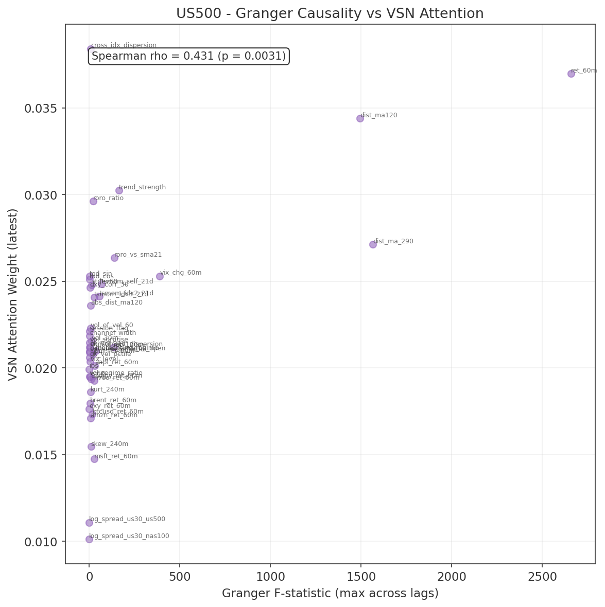
Over half the feature–lag combinations are statistically significant for US30 and US500 after conservative multiple-testing correction. NAS100 is slightly lower, consistent with its higher idiosyncratic noise from concentrated technology exposure.

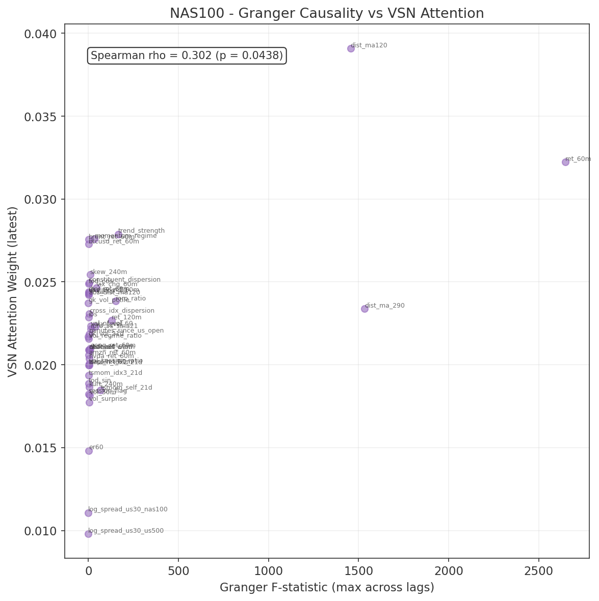
Top features by F-statistic (consistent across all three indices):

Rank	Feature	F-stat (US30)	F-stat (US500)	F-stat (NAS100)
1	ret_60m	> 2600	> 2600	> 2600
2	dist_ma_290	> 1500	> 1500	> 1500
3	dist_ma120	> 1450	> 1450	> 1450
4	trend_strength	~165	~165	~165
5	ret_120m	~143	~138	~130

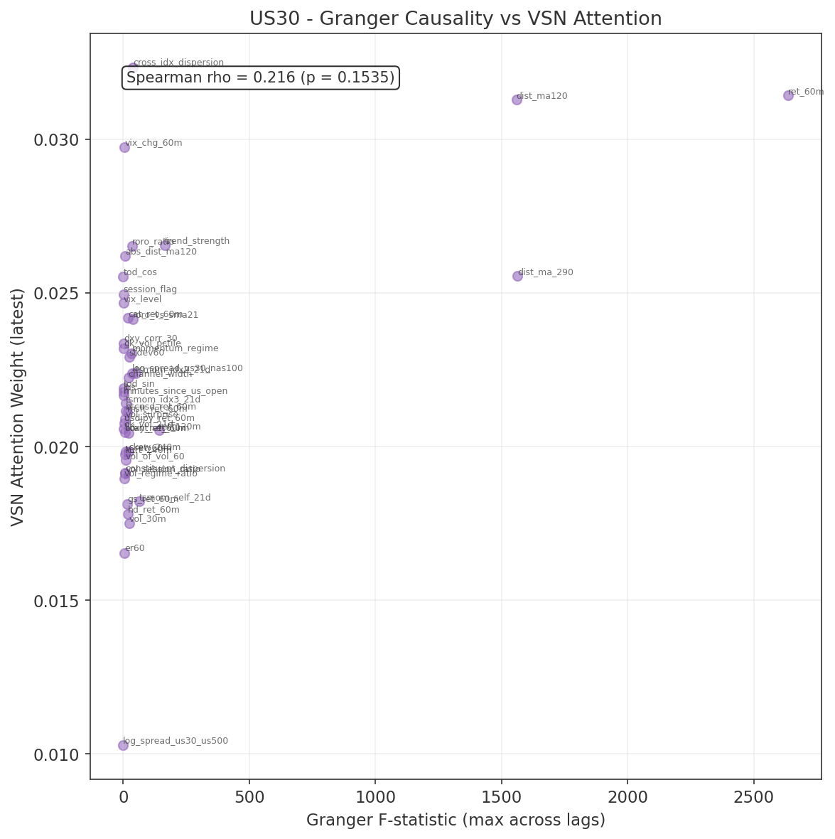
All five are own-instrument features from Group 1 (core price dynamics). The dominance of ret_60m is expected: the target is forward 60-minute returns, and the autoregressive component of returns at this horizon is well-documented. The two moving-average distance features capture trend persistence at different time scales.

Features significant in all three indices (24 of 45):

abs_dist_ma120, brent_ret_60m, channel_width, constituent_dispersion, cross_idx_dispersion, dist_ma120, dist_ma_290, kurt_240m, momentum_regime, msft_ret_60m, ret_120m, ret_60m, roro_ratio, roro_vs_sma21, skew_240m, stdev60, trend_strength, tsmom_idx3_21d, tsmom_self_21d, vol_30m, vol_of_vol_60, vol_regime_ratio, vol_session_ratio, vol_surprise.

This set spans all five feature groups: core price dynamics (Group 1), volatility and higher moments (Group 2), cross-index signals from the gap studies (Group 3), cross-asset features (Group 4), and microstructure proxies (Group 5). The cross-index features (cross_idx_dispersion, roro_ratio, roro_vs_sma21, tsmom signals) all pass, confirming that the Phase 2 gap study findings survive formal causality testing.

Features not significant on any index after Bonferroni correction:

er60, tod_sin, tod_cos, ibs, gk_vol_pctile, session_flag, dxy_corr_30, and several individual constituent returns. The time-of-day features (tod_sin, tod_cos, session_flag) are deterministic functions of the clock and contain no stochastic information about returns. IBS and gk_vol_pctile are bounded indicators that operate conditionally (IBS predicts only within specific volatility regimes, as shown in Gap Study #8). The log-spread features (log_spread_us30_us500, log_spread_us30_nas100) were borderline, consistent with the slow mean-reversion documented in Gap Study #1.

Key Findings

1. Majority of features pass Granger causality. Over 50% of feature-lag combinations are significant after Bonferroni correction for US30 and US500, and 42% for NAS100. The feature set carries genuine linear predictive content for forward 60-minute returns.
2. Own-instrument features dominate. The top 5 features by F-statistic are all from Group 1 (core price dynamics), with ret_60m and the moving-average distance features showing the strongest causal signal across all three indices.
3. Cross-index features validated. All Phase 2 gap-study-derived features (cross_idx_dispersion, roro_ratio, roro_vs_sma21, tsmom signals) pass the Granger test, confirming that the empirical gap study findings survive formal causality testing.
4. Non-significant features retained as VSN validation. Features that fail Granger causality were deliberately retained as a validation mechanism for the Variable Selection Network. If the VSN works correctly, it should independently learn to downweight these features. The Run 1 training results (Section 7.5) confirm this: log_spread_us30_us500 (not Granger-causal) received the lowest VSN attention, while the top Granger-causal features received the highest. This correspondence provides independent validation that the VSN is working as intended.

Charts

7. Phase 3: Neural Net Model Development

7.1 Data Inventory

This section documents the data available for model development. All three index models share a common training window, cross-asset feature set, and chronological train/validation/test split. The binding constraint on the common window is META, whose M1 data begins on 2021-06-30.

Common Training Window

Parameter	Value
Window	2021-07-01 to 2026-03-17 (~4.7 years)
Binding constraint	META (starts 2021-06-30)
Bar frequency	M1 (1-minute OHLCV)
Source	MT5 CFD data + Databento XNAS backfill (TLT, META)

Target Indexes

Each model predicts the forward 60-minute return using a double-barrier label (up/down/hold).

Instrument	Full Span	M1 Rows
US30 (DJIA)	2020-08 to 2026-03	1,982,699
US500 (S&P 500)	2018-05 to 2026-03	2,743,872
NAS100 (Nasdaq 100)	2018-05 to 2026-03	2,792,656

Cross-Asset Instruments

The following instruments provide cross-asset features for all three models.

Instrument	Full Span	M1 Rows	Feature Use
VIX	2018-05 to 2026-03	760,033	Fear gauge, vol regime
DXY (Dollar Index)	2018-12 to 2026-03	2,194,608	Dollar strength
USDJPY	2008-09 to 2026-03	2,133,765	Carry trade / risk proxy
BTCUSD	2017-06 to 2026-03	2,325,662	Risk appetite proxy
XAUUSD (Gold)	2018-05 to 2026-03	2,802,955	Safe haven flow
BRENT (Crude Oil)	2016-01 to 2026-03	1,839,566	Energy / inflation proxy
TLT (20Y+ Treasury Bond ETF)	2018-05 to 2026-02	971,662	Bond proxy, equity/bond rotation

Constituent Stocks

The top 5 constituents per index provide 60-minute returns as features and intra-index dispersion measures. Several stocks appear in multiple index models.

Index	Top 5 Constituents
US30	GS, MSFT, HD, CAT, V
NAS100	AAPL, MSFT, NVDA, AMZN, GOOG
US500	AAPL, MSFT, NVDA, AMZN, META (binding constraint)

AAPL, MSFT, NVDA, and AMZN appear in both the NAS100 and US500 constituent sets. MSFT also appears in the US30 set, making it the only stock present across all three models.

Train / Validation Split

All splits are strictly chronological with no overlap. No data from the validation set is used during training or hyperparameter selection.

Split	Period	Duration	Share
Train	2021-07-01 to 2025-06-30	4.0 years	83%
Validation	2025-07-01 to 2026-03-17	~8.5 months	17%

All splits are strictly chronological. The validation set includes the 2025 tariff volatility regime. The real out-of-sample test is live execution on MT5.

Data Quality Notes

• All files are clean M1 bars, verified via interval analysis (no duplicate timestamps, no gaps exceeding expected market closures).
• Missing minutes in lower-volume stocks reflect thin liquidity during off-peak hours, not data errors. These gaps are expected and handled during feature construction.
• Stock constituents only trade 13:30 to 20:00 UTC (US cash session). Outside these hours, constituent features are forward-filled from the last available bar.

7.2 Feature Specification

Each model receives approximately 45 features per M1 bar, organised into five groups. Every feature is justified either by Phase 1 literature or by Phase 2 empirical results. The prediction target is the forward 60-minute return, encoded via double-barrier labelling (up / down / hold).

Group 1: Own-Instrument Core (18 features)

These features are proven predictors from the XAUUSD base model, adapted for equity indices. They capture returns, volatility structure, trend quality, distribution shape, and time-of-day cyclicality.

Feature	Formula / Definition	Rationale
ret_60m	$\ln(p_t / p_{t-60})$	Recent return momentum
ret_120m	$\ln(p_t / p_{t-120})$	Medium-horizon return
dist_ma120	$(p_t - \text{MA}_{120}) / \text{MA}_{120}$	Signed distance from 2h MA
dist_ma290	$(p_t - \text{MA}_{290}) / \text{MA}_{290}$	Signed distance from session MA
stdev60	$\sigma(\text{ret}_{1m}, w{=}60)$	Realised volatility (1h)
vol_30m	$\sigma(\text{ret}_{1m}, w{=}30)$	Short-window volatility
vol_session_ratio	$\sigma_{30m} / \sigma_{\text{session}}$	Intraday vol regime
vol_of_vol_60	$\sigma(\sigma_{30m}, w{=}60)$	Volatility clustering intensity
vol_regime_ratio	$\sigma_{60m} / \sigma_{240m}$	Short vs long vol ratio
vol_surprise	$(\sigma_{30m} - \mu_{\sigma,240}) / \sigma_{\sigma,240}$	Vol Z-score (surprise detection)
channel_width	$Q_{0.95} - Q_{0.05}$ (rolling 120 bars)	Quantile regression channel
skew_240m	Rolling skewness, $w{=}240$	Return distribution asymmetry
kurt_240m	Rolling kurtosis, $w{=}240$	Tail heaviness
er60	$|\Delta p_{60}| / \sum_{i=1}^{60}|\Delta p_i|$	Kaufman efficiency ratio $[0,1]$
momentum_regime	Binary: MA crossover aligned with return sign	Trend alignment indicator
trend_strength	$\text{sign}(\text{ret}_{60m}) \times \text{ER}_{60} \times |\text{ret}_{60m}| / \sigma_{60m}$	Signed ER x normalised magnitude
tod_sin	$\sin(2\pi \cdot \text{minute} / 1440)$	Cyclical time-of-day encoding
tod_cos	$\cos(2\pi \cdot \text{minute} / 1440)$	Cyclical time-of-day encoding

Group 2: Cross-Index Features (11 features)

Every feature in this group traces directly to a specific Phase 2 gap study. These encode cross-index momentum, risk regime, volatility state, and structural spread dynamics.

Feature	Formula / Definition	Source
tsmom_self_21d	$\text{sgn}\bigl(\sum_{i=1}^{21} r_i\bigr)$, trailing monthly return	Study #4 (TSMOM)
tsmom_idx2_21d	Same, for second index	Study #4
tsmom_idx3_21d	Same, for third index	Study #4
roro_ratio	$\ln(\text{NAS100} / \text{US30})$	Study #2 (RORO)
roro_vs_sma21	Binary: RORO ratio above/below 21d SMA	Study #2
gk_vol_21d	Garman-Klass volatility, 21-day rolling	Study #5 (Vol regime)
gk_vol_pctile	Expanding percentile rank of GK vol	Study #5
ibs	$(\text{close} - \text{low}) / (\text{high} - \text{low})$, daily	Study #8 (conditional on vol regime)
cross_idx_dispersion	$\sigma(\text{ret}_{60m}^{(i)})$ across all 3 indices	Study #4 (rotation signal)
log_spread_us30_us500	$\ln(\text{US30}) - \ln(\text{US500})$	Study #1 (novel)
log_spread_us30_nas100	$\ln(\text{US30}) - \ln(\text{NAS100})$	Study #1 (novel)

Group 3: Cross-Asset Macro (7 features)

Macro features capture risk appetite, dollar strength, carry dynamics, and energy/inflation pressure. Three candidates were dropped due to insufficient history in the common training window.

Feature	Formula / Definition	Rationale
vix_level	VIX spot value	Fear gauge level
vix_chg_60m	$\Delta\text{VIX}_{60m}$	VIX momentum (shock detection)
dxy_ret_60m	$\ln(\text{DXY}_t / \text{DXY}_{t-60})$	Dollar strength
dxy_corr_30	Rolling 30-bar correlation(index, DXY)	Dollar correlation regime
usdjpy_ret_60m	$\ln(\text{USDJPY}_t / \text{USDJPY}_{t-60})$	Yen carry proxy
btcusd_ret_60m	$\ln(\text{BTCUSD}_t / \text{BTCUSD}_{t-60})$	Crypto risk appetite
brent_ret_60m	$\ln(\text{BRENT}_t / \text{BRENT}_{t-60})$	Energy / inflation proxy

Dropped instruments: TLT (only 3 months of M1 data in common window), LQD (3 months), USOIL (4 months; replaced by BRENT which has full coverage from 2016).

Group 4: Constituent Returns (6 features per model)

The top 5 constituents by index weight provide 60-minute returns as individual features. A sixth feature, constituent_dispersion, measures intra-index disagreement. The constituent set differs per model.

Model	Top-5 Constituents	Dispersion Feature
US30	GS, MSFT, HD, CAT, V	$\sigma(\text{ret}_{60m}^{(k)})$, $k \in \{1..5\}$
NAS100	AAPL, MSFT, NVDA, AMZN, GOOG	$\sigma(\text{ret}_{60m}^{(k)})$, $k \in \{1..5\}$
US500	AAPL, MSFT, NVDA, AMZN, JPM	$\sigma(\text{ret}_{60m}^{(k)})$, $k \in \{1..5\}$

Group 5: Intraday Seasonality (2 features)

Feature	Definition	Rationale
session_flag	Asia = 0, London = 1, US = 2	Session regime (liquidity + volatility differ by session)
minutes_since_us_open	Minutes elapsed since 13:30 UTC	Distance from highest-activity period

Feature Count Summary

Group	Features
Own-Instrument Core	18
Cross-Index	11
Cross-Asset Macro	7
Constituent Returns	6
Intraday Seasonality	2
Total	44

Normalisation

Method	Applied To	Window
rolling_z	Continuous non-stationary features (returns, distances, vol levels)	$w = 1440$ (24 hours)
zscore (expanding)	Stable distributions (GK vol percentile, kurtosis)	Expanding from start of training set
passthrough	Bounded or naturally scaled features (ER, IBS, session_flag, tod_sin/cos)	None

Lookahead Prevention

All features are strictly causal. Daily IBS uses the previous completed day only. TSMOM signals use completed daily returns only. No feature reads future prices. Rolling windows use only data available at time $t$, with no forward-looking statistics.

Feature Provenance

The following table summarises the link between cross-index / cross-asset features and the Phase 2 gap studies that justified their inclusion.

Feature(s)	Phase 2 Study	Key Finding
tsmom_self_21d, tsmom_idx2_21d, tsmom_idx3_21d, cross_idx_dispersion	Study #4 (Cross-index momentum)	TSMOM rotation: Sharpe 1.27
roro_ratio, roro_vs_sma21	Study #2 (RORO ratio)	Valid vol regime indicator; 20-28% higher vol in risk-off
gk_vol_21d, gk_vol_pctile	Study #5 (Vol regime selection)	MR works in high-vol NAS100 (Sharpe 0.99)
ibs	Study #8 (IBS/RSI replication)	Conditional on vol regime only; fails in aggregate
log_spread_us30_us500, log_spread_us30_nas100	Study #1 (PW vs CW divergence)	Novel; extreme Z-score reversion observed
session_flag, minutes_since_us_open	Study #9 (Intraday seasonality)	Vol and momentum differ by session

7.3 Normaliser Selection

Why Normalisation Matters

Raw features can drift across regimes — VIX level, channel width, and kurtosis all exhibit non-stationary behaviour over months-long windows. Without normalisation, drifting features dominate the neural net's gradient updates, causing training instability or the model learning spurious regime-dependent patterns. But normalisation can also destroy information, particularly in features where the raw scale is the signal. Absolute volatility levels, dispersion magnitudes, and vol ratios all carry meaning in their raw units that z-scoring can erase.

Methodology

Each of the 36 continuous features was tested under three normalisation strategies on the validation set (2025-07 to 2026-03):

Strategy	Description
raw	No normalisation (baseline)
rolling_z	Causal 30-day rolling $3\sigma$ clip + z-score
rolling_winsor_z	Causal 30-day rolling 1st–99th percentile clip + z-score

Static normalisation (global mean/std computed over the full dataset) was excluded because it leaks regime information and fails on drifting features — a model trained during a low-VIX period would see systematically biased inputs during a high-VIX regime.

Decision rule:

1. Compute gain = AUC(rolling_z) $-$ AUC(raw) for each feature on each index.
2. Average across all 3 indices.
3. If avg gain $< -0.001$ AND rolling_z hurts on at least 2/3 indices → passthrough.
4. If already bounded/binary → passthrough.
5. Otherwise → rolling_z (safe default for drift protection).

The rolling_winsor_z strategy (percentile clip instead of $\sigma$-clip) was never chosen. Gains over rolling_z were marginal and inconsistent across the three indices.

Final Split: 17 Passthrough / 28 Rolling Z-Score

The per-feature decision rule produces a clear split: 17 features are passed through without normalisation, and 28 features use rolling_z.

Passthrough Features (17)

These fall into two categories:

Bounded/binary (9):

• er60 $[0,1]$
• momentum_regime $\{0,1\}$
• tod_sin $[-1,1]$, tod_cos $[-1,1]$
• roro_vs_sma21 $\{0,1\}$
• gk_vol_pctile $[0,1]$
• ibs $[0,1]$
• dxy_corr_30 $[-1,1]$
• session_flag $\{0,1,2\}$
• minutes_since_us_open $[0,1]$

Scale-is-signal (8):

• ret_60m — naturally mean-zero and stationary
• stdev60 and vol_30m — realised volatility is stationary; raw level encodes regime
• vol_session_ratio and vol_surprise — self-normalising ratios
• gk_vol_21d — daily Garman-Klass vol, naturally bounded (avg gain $-0.0022$)
• cross_idx_dispersion — strongest negative (avg gain $-0.0037$)
• vix_level — highest drift (2.72) but rolling_z kills regime signal (avg gain $-0.0037$)

Rolling Z-Score Features (28)

All other continuous features use rolling_z. Key beneficiaries:

Feature	Avg $\Delta$AUC	Notes
kurt_240m	+0.0020	High drift 1.67–1.75
skew_240m	+0.0020	—
channel_width	+0.0013	High drift 4.5–4.8
tsmom_idx3_21d	+0.0013	Consistently positive all 3 indices
log_spread_us30_us500	+0.0013	Drifts by construction
abs_dist_ma120	+0.0009	Consistently positive all 3 indices
dxy_ret_60m	+0.0006	Consistently positive all 3 indices
All constituent stock returns: rolling_z protects against earnings/split outliers

Cross-Instrument Results

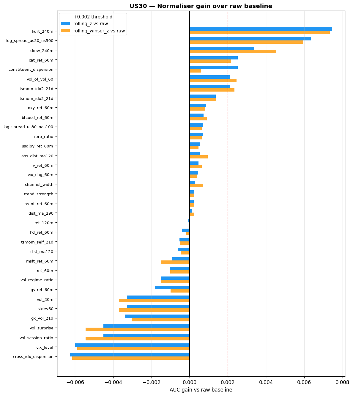
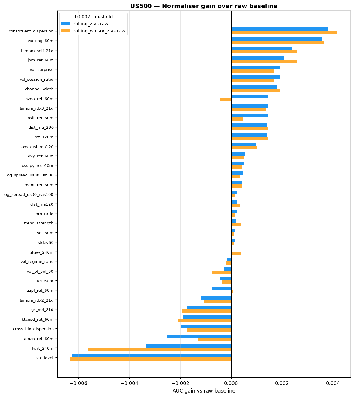
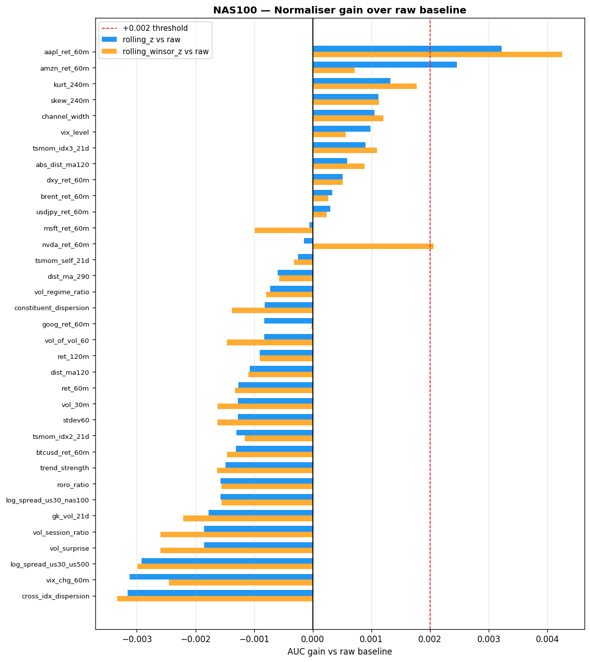
The following tables summarise AUC gains from rolling_z versus raw on each index. A positive value means normalisation helped; a negative value means the raw scale carried predictive information that z-scoring destroyed.

Features where rolling_z helps most (AUC gain $> 0.002$ on at least one index):

Feature	US30 $\Delta$AUC	NAS100 $\Delta$AUC	US500 $\Delta$AUC	Drift Score
kurt_240m	+0.0074	+0.0018	—	1.67 / 1.75
log_spread_us30_us500	+0.0063	—	—	—
skew_240m	+0.0045	—	—	—
aapl_ret_60m	—	+0.0043	—	—
constituent_dispersion	—	—	+0.0042	—
vix_chg_60m	—	—	+0.0036	—
tsmom_self_21d	—	—	+0.0026	—
amzn_ret_60m	—	+0.0025	—	—

Features where rolling_z hurts most (raw scale carries predictive information):

Feature	US30 $\Delta$AUC	NAS100 $\Delta$AUC	US500 $\Delta$AUC
cross_idx_dispersion	-0.0061	-0.0032	—
vix_level	-0.0059	—	-0.0063
vol_session_ratio	-0.0045	—	—
vol_surprise	-0.0045	—	—
vol_30m	-0.0033	—	—
stdev60	-0.0033	—	—

Final Decision

Normaliser	Count
passthrough	17 (9 bounded + 8 scale-dependent)
rolling_z	28
Total	45

VIX note: VIX has the highest drift (2.72) but is passthrough. If training instability is observed, $\log(\text{VIX})$ is a fallback that is more stationary while preserving regime information.

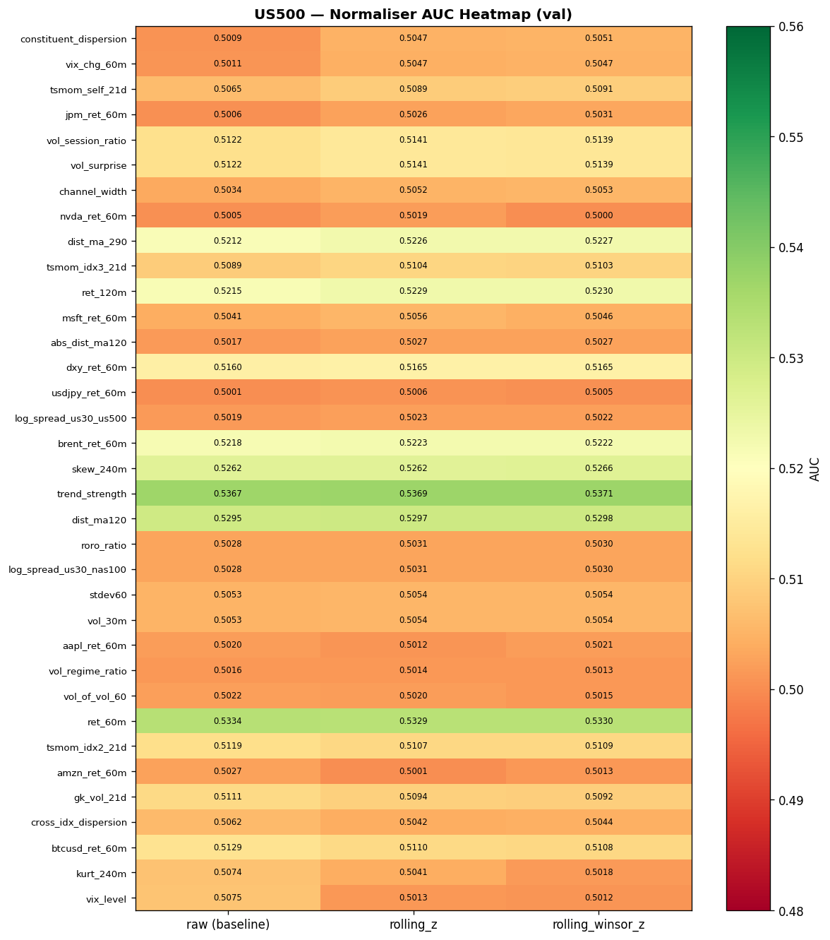
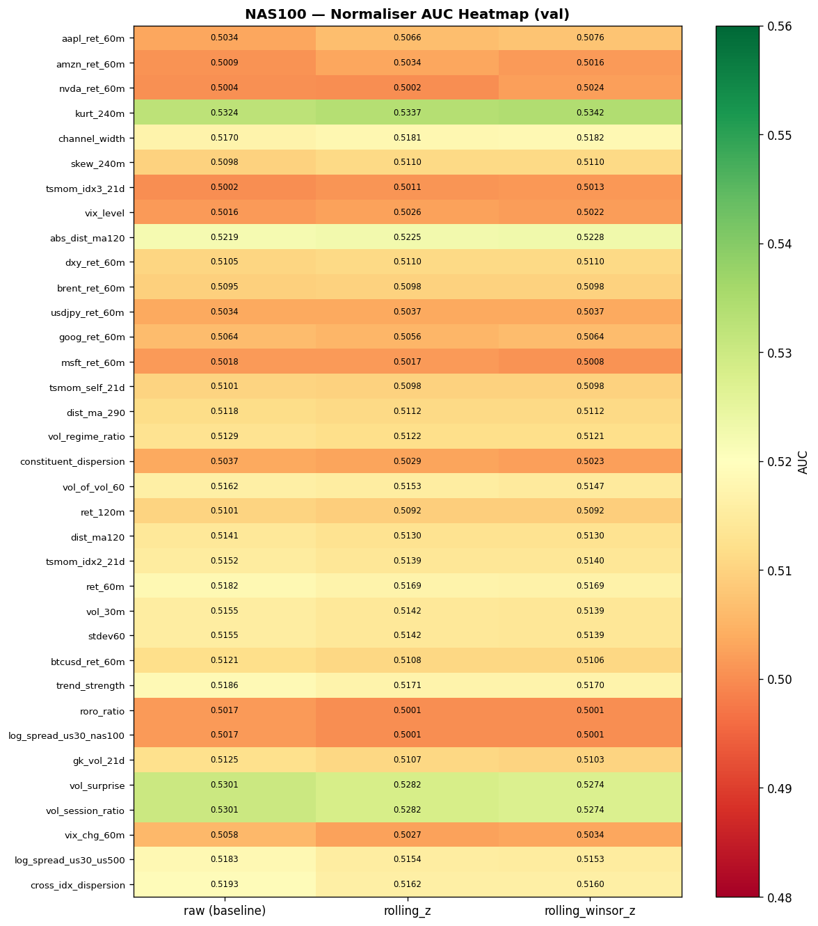
Normaliser AUC Heatmaps

The following heatmaps show directional AUC (one-vs-rest classifier on the double-barrier label) for each feature under each normalisation strategy. Green cells indicate AUC above baseline (0.5); darker shading indicates stronger signal.

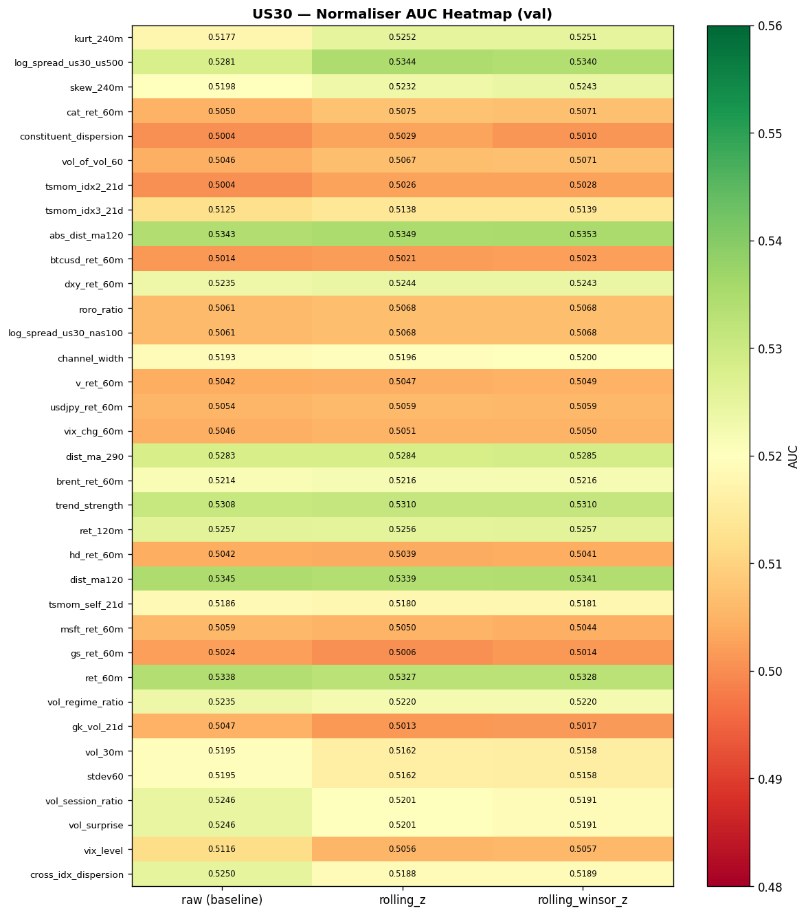
Expand: US500 and NAS100 normaliser heatmaps

AUC Improvement from Rolling Z-Score

Bar charts showing the per-feature AUC change when switching from raw to rolling_z. Positive bars (green) indicate features that benefit from normalisation; negative bars (red) indicate features where the raw scale carries signal.

Expand: US500 and NAS100 AUC improvement charts

Drift Score vs. Normalisation AUC Gain

Scatter plots of feature drift score (x-axis, measured as the ratio of inter-month variance to intra-month variance) against AUC gain from rolling_z (y-axis). Features in the upper-right quadrant are high-drift features that benefit from normalisation. Features in the lower-right are high-drift features where normalisation hurts — these are the scale-dependent features (VIX level, dispersion) where drift is real but informative.

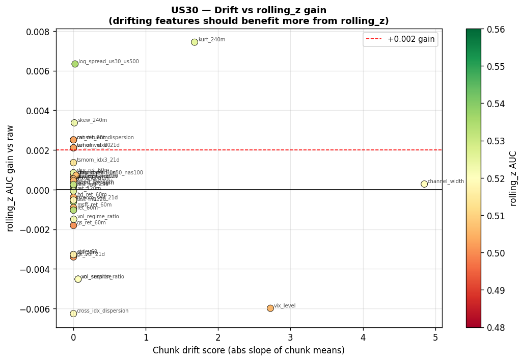
Expand: US500 and NAS100 drift-vs-gain scatter plots

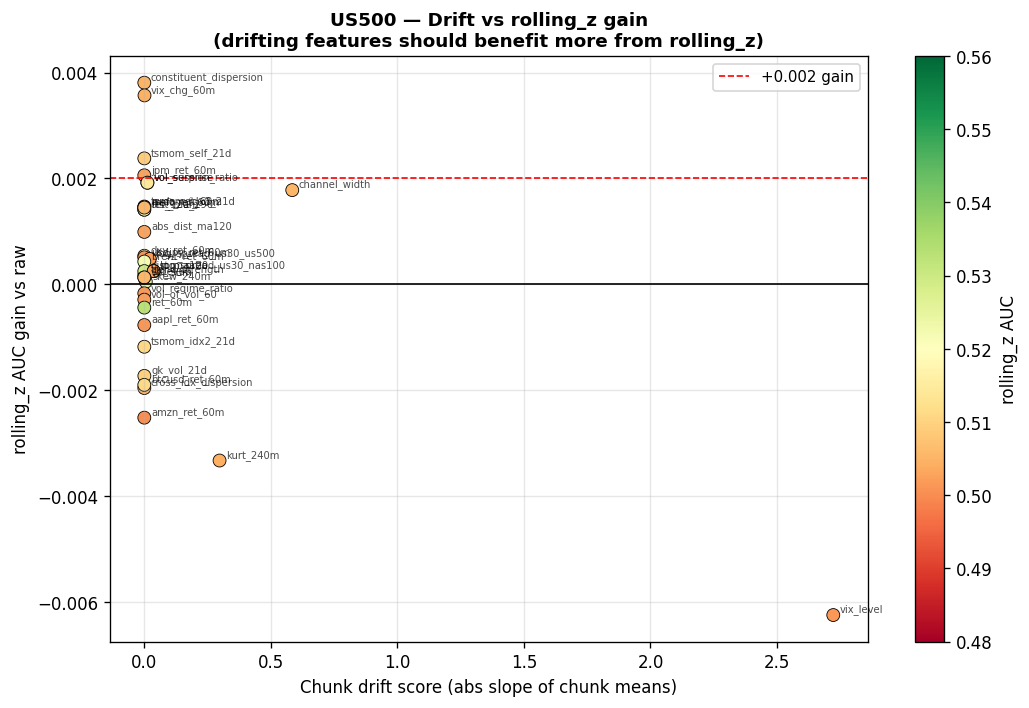
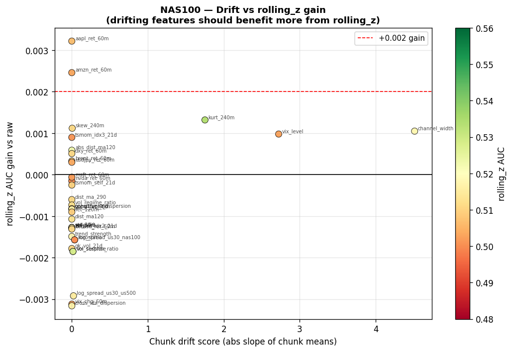
7.4 Model Configuration

Target Variable

The target is the forward 60-minute return, labelled via symmetric double-barrier classification. Every bar receives a directional prediction — there is no trade/no-trade gate at the model level. The barrier is set per-index to account for different price levels:

Index	Barrier	Approx %	Rationale
US30	\$100	~0.24%	DJIA ~42,000
US500	\$30	~0.52%	S&P 500 ~5,800
NAS100	\$200	~1.0%	NASDAQ-100 ~20,000

Bars where price stays within the barrier for the full 60-minute horizon are labelled "hold."

Trading Costs

Index	Spread
US30	\$1.20
US500	\$0.50
NAS100	\$2.00

Architecture: VSN + TCN + Transformer

The model pipeline is: Features → Variable Selection Network (VSN) → Temporal Convolutional Network (TCN) → Transformer encoder → prediction heads. The VSN produces a dense embedding from the raw feature vector at each timestep; the TCN extracts local temporal patterns from the embedding sequence; the Transformer captures global dependencies across the full window. The adaptive denoise filter (used in the XAUUSD base model) is disabled here because index composites already smooth microstructure noise inherent in single-instrument tick data.

Four parallel ContextTCNTransformer modules operate at different temporal scales:

Stream	Bars	Duration	Purpose
Short	60	1 hour	Immediate momentum
Mid	120	2 hours	Medium-term trend
Long	240	4 hours	Full session context
Slow	720	30 days	Macro regime (H1 resampled)

The slow stream resamples to H1 bars (720 H1 bars = 30 trading days) for long-range regime context without inflating sequence length.

Variable Selection Network (VSN)

The VSN is a learned, per-timestep soft feature gate based on the Variable Selection Network introduced by Lim et al. (2021) in the Temporal Fusion Transformer. Given $F$ input features at each timestep, the VSN produces softmax-normalised importance weights via a selector MLP, then projects the weighted features into a dense embedding of dimension $E$. This allows the model to suppress noisy or irrelevant features on a bar-by-bar basis rather than treating all 44 inputs equally.

The VSN computes two complementary paths and combines them via element-wise addition:

Path	Computation	What It Captures
Value path	$x \odot w \rightarrow \text{Linear}(F, E)$	How much each feature contributes (magnitude-aware)
Prototype path	$w^\top \cdot \text{Prototypes}(F, E)$	Which features are active (identity-aware)

The value path multiplies each raw feature by its importance weight and projects the result to the embedding dimension. The prototype path takes the dot product of the weight vector with a learnable prototype matrix, producing an embedding that reflects which features are selected regardless of their magnitude. The element-wise sum passes through LayerNorm to produce the final embedding fed to the TCN.

Why VSN before TCN. Each layer in the pipeline operates on a different axis and is blind to what the others handle:

Component	Operates Across	Learns	Blind To
VSN	Features ($F$ axis)	Which features matter at this timestep	Temporal patterns
TCN	Time ($T$ axis)	Local temporal patterns (15-bar kernel)	Feature quality
Transformer	Time ($T$ axis)	Global dependencies across full window	Local patterns

By composing VSN → TCN → Transformer, each layer handles what it does best. The VSN says “at this bar, dxy_ret_60m and vol_surprise are the key inputs; suppress noisy constituents.” The TCN says “over the last 15 bars of those selected features, there is momentum acceleration.” The Transformer says “across the full window, trend context supports this direction.”

Why not feed raw features directly to the TCN. The 44 features range from near-random (AUC 0.5004) to meaningfully predictive (AUC 0.5367). Without the VSN, the TCN treats every feature channel equally, wasting capacity on noise. Furthermore, feature importance is regime-dependent: momentum features matter during trends, while volatility features matter in mean-reverting markets. The VSN adapts per-timestep, allowing the downstream TCN to operate on a cleaned, regime-appropriate representation.

VSN hyperparameters:

Parameter	Value	Notes
Hidden dim	64	Selector MLP hidden size
Dropout	0.15	Matches model-wide dropout
Context dim	0	No regime context ($K = 1$)

Parameter cost: approximately 11,648 parameters total (selector MLP ~5,760, value projection ~2,880, prototypes ~2,880, LayerNorm ~128). This is negligible relative to the Transformer encoder and does not meaningfully increase training time or memory.

VSN Entropy Regularisation

Without regularisation, the VSN softmax gate can collapse, concentrating all attention on one or two features and ignoring the rest. This wastes the 45-feature design, overfits to a narrow signal, and suppresses jointly informative but individually weak features.

We add the Shannon entropy of the VSN weights to the loss as a regularisation term:

$$H(\mathbf{w}_t) = -\sum_{i=1}^{F} w_{t,i} \log(w_{t,i})$$

where $\mathbf{w}_t$ is the $F$-dimensional softmax weight vector at timestep $t$. Maximum entropy ($\log F \approx 3.8$ for 45 features) corresponds to uniform attention; minimum entropy (0) corresponds to complete collapse onto a single feature.

The entropy is averaged across all timesteps, batch samples, and all four streams, then subtracted from the loss. Higher entropy (more diverse feature usage) reduces the loss, nudging the model toward balanced attention.

Parameter	Value	Notes
$\lambda_{\text{vsn}}$	0.002	Deliberately small: direction loss (~1.0) dominates; entropy term (~0.006) acts as a gentle nudge

Scenario	Entropy	Effect on Loss
Uniform attention (all 45 features)	~3.8	Loss reduced by ~0.0076
Concentrated on 5 features	~1.6	Loss reduced by ~0.0032
Collapsed to 1 feature	~0.0	No entropy benefit

The model learns to balance concentrating on the most predictive features (to minimise direction loss) against maintaining enough diversity to earn the entropy bonus. If entropy drops below ~1.0 during training, the VSN is collapsing and $\lambda_{\text{vsn}}$ should be increased.

TCN + Transformer Hyperparameters

Parameter	Value
Embedding dimension	128
Layers	1
Attention heads	4 (32 per head)
Dropout	0.15
TCN channels	64
TCN kernel	15 (15-min receptive field)

Training Configuration

Parameter	Value	Notes
Epochs	50	With warmup + cosine schedule
Batch size	512	Fits GPU with 4 streams
Learning rate	$3 \times 10^{-4}$	Standard Transformer LR
Weight decay	0.005	Regularisation
Expected PnL loss	Disabled	Use supervised BCE/CE for direction
Regime clusters	$K = 1$	No clustering; learn direction first

Design Decisions

$K = 1$ regime clustering. A single prediction head is used. Regime clustering with $K > 1$ fragments the already limited data across multiple heads, each seeing a fraction of the training samples. The model learns direction first; regime specialisation can be added once the base model demonstrates signal.

No trade gate. Every bar receives an up/down/hold prediction. The trade/no-trade decision is made by the executor based on confidence thresholds, not by the model. This keeps the model focused on directional classification and avoids conflating two separate objectives in a single output.

Dropout 0.15. Higher than the typical 0.05–0.10 used in NLP Transformers, because financial features are substantially noisier than language tokens. This value was validated on the XAUUSD base model, where lower dropout (0.05) led to overfitting on training data.

Learning rate $3 \times 10^{-4}$. Standard for Transformer architectures. Higher rates (e.g., $10^{-2}$) cause catastrophic early updates that destroy the attention mechanism before it can learn meaningful patterns. Lower rates (e.g., $10^{-5}$) converge too slowly within 50 epochs.

Data Pipeline

7.5 Training Results

Cross-Index Summary

The table below consolidates all training runs across the three indices, highlighting the Run 2 improvements.

Index	Run	Best Epoch	Val Acc	Val Loss	Class Gap	VSN Ratio	Status
US30	Run 1	3	67.8%	0.933	6.0pp	3.1x	Superseded
US30	Run 2	4	68.4%	0.891	1.6pp	2.0x	Deploy candidate
US30	Run 3a	3	55.7%	1.562	16.7pp	—	Failed — aux loss dominance
US30	Run 3b	—	55.4%	—	—	—	Failed — capacity bottleneck
US30	Run 3c	8	55.3%	2.964	—	—	Failed — position-agnostic VSN
US30	Run 3d	5	70.5%	1.029	4.7pp	—	New best
US500	Run 1	7	63.1%	1.649	15.5pp	3.8x	Superseded
US500	Run 2	5	62.0%	1.349	4.9pp	2.0x	Superseded
US500	Run 3d	2	68.1%	—	18.3pp	—	New best (+6.1pp)
NAS100	Run 1	5	68.9%	0.792	0.6pp	2.2x	Superseded
NAS100	Run 2	3	68.9%	0.783	20.2pp*	1.8x	Superseded
NAS100	Run 3d	2	68.7%	—	11.2pp	—	No improvement; 4-stream preferred
US30	Run 3e	—	—	—	—	—	Failed — weighted fallback poisoned training
US500	Run 3e	—	—	—	—	—	Failed — weighted fallback poisoned training
US30	Run 3f	1	67.6%	—	—	—	First profitable backtest: +$82,843
US500	Run 3f	—	—	—	—	—	Unprofitable — spread cost prohibitive
US30	Run 3h	1	64.7% (tradeable)	—	—	—	+$37,266; 3-class HOLD; edge in 00-06 UTC
US30	Run 3i	1	—	—	—	—	+$66,370; asymmetric barriers; UP 44.7% / DOWN 29.6%
US30	Run 3j	3	—	—	—	—	+$79,938; MAE smoothing eliminated epoch cliff; short WR 59.3%
US30	Run 3k	1	—	—	—	—	+$28,931; symmetric barriers hurt shorts; softmax zero-sum confirmed
US30	Run 3L Short	7	—	—	—	—	+$127,633; PF 1.90; short specialist; best result in study
US30	Run 3L Long	1	—	—	—	—	-$13,690; barrier labels fundamentally wrong for longs
US30	Run 3M	333	—	—	—	—	-$47,413; return labels; dip-buy signal discovered
US30	Run 3N	30	—	—	—	—	+$4,683; first profitable longs; dip-buy model
US30	Run 3O	43	—	—	—	—	+$4,157; wider TP/SL; similar PnL, fewer trades

*NAS100 Run 2 epoch 3 has a transient bullish bias (20.2pp gap) that resolves to 0.7pp by epoch 5. For balanced deployment, use epoch 5 (68.3% accuracy).

Note: US500 and NAS100 results are invalidated by the barrier calibration flaw discovered in Section 7.11. Their barriers (US500 $90, NAS100 $200) were 27-29x the median hourly move, producing 0% real barrier hits. 100% of training labels were fallback close-to-close direction, not barrier-based signal. US30 ($100 barrier, 3.7x ratio, 21% hit rate) was partially valid but suboptimal. Retraining with corrected barriers is required.

US30 — Run 1 & Run 2 Detail

US30 — Run 1 (Diagnostic)

Simulated Results — All results in this section are from simulated training and validation on historical data. They do not represent live trading performance. Validation accuracy measures directional prediction on held-out bars (2025-07 to 2026-03) that were not seen during training.

This is the first training run for the US30 model. The purpose is diagnostic: confirm the architecture can learn directional signal, identify failure modes, and calibrate regularisation for subsequent runs. The results reveal severe overfitting but also genuine directional signal in the validation set.

Configuration

Parameter	Value
Target	US30
Barrier	$100
Spread	$1.20
Batch size	512
Learning rate	$3 \times 10^{-4}$ (warmup + cosine)
Epochs	18 / 50 (early termination)
VSN entropy $\lambda$	0.001 (later increased to 0.002)
Train period	2021-07 to 2025-06
Validation period	2025-07 to 2026-03

Headline Results

Metric	Value
Best validation loss	0.933 (Epoch 3)
Best validation direction accuracy	67.8% (Epoch 3)
Final validation direction accuracy	64.9% (Epoch 18)
Final train direction accuracy	92.0% (Epoch 18)
Coverage	95.7%
$p_{\text{up}}$ std	0.438 (healthy, no hedging)
VSN entropy	3.635 (max 3.81)

Key Observations

Epoch 3 is the sweet spot. Validation loss hits its minimum (0.933) and validation accuracy peaks (67.8%) at epoch 3, during the warmup phase when the effective learning rate is approximately $1.4 \times 10^{-4}$. Everything after epoch 3 is overfitting. This pattern is consistent with the XAUUSD base model experience: Transformers on noisy financial data find their best generalisation early, before the optimiser has enough capacity to memorise training noise.

Severe overfitting from epoch 4 onwards. Validation loss increased 143% from epoch 3 to epoch 18 (0.93 to 2.27). The train–validation accuracy gap grew from 6.7 percentage points (epoch 3: 74.5% train, 67.8% val) to 27.1 percentage points (epoch 18: 92.0% train, 64.9% val). The model memorised the training set.

Directional signal is real. A validation accuracy of 67.8% is well above the 50% random baseline and above the ~55% threshold typically required for profitability after transaction costs. DOWN accuracy (70.5%) exceeds UP accuracy (64.5%), indicating a slight bearish bias in the model's learned representations. This asymmetry may reflect the validation period (2025-07 to 2026-03) containing more volatile down-moves that are easier to predict.

VSN is healthy. Entropy decreased from 3.78 to 3.64 (theoretical maximum 3.81 for 45 features), meaning the Variable Selection Network learned to differentiate feature importance without collapsing to a small subset. The entropy regularisation term ($\lambda = 0.001$) served its purpose.

No gradient issues. Gradient norms remained stable throughout all 18 epochs. No exploding or vanishing gradients were observed, confirming the warmup + cosine annealing schedule is appropriate for this architecture.

Coverage ramped quickly. Coverage (fraction of bars where the model produces a non-hold prediction with sufficient confidence) increased from 60% at epoch 1 to 96% by epoch 6. The model became confident on nearly all directional bars early in training.

Charts

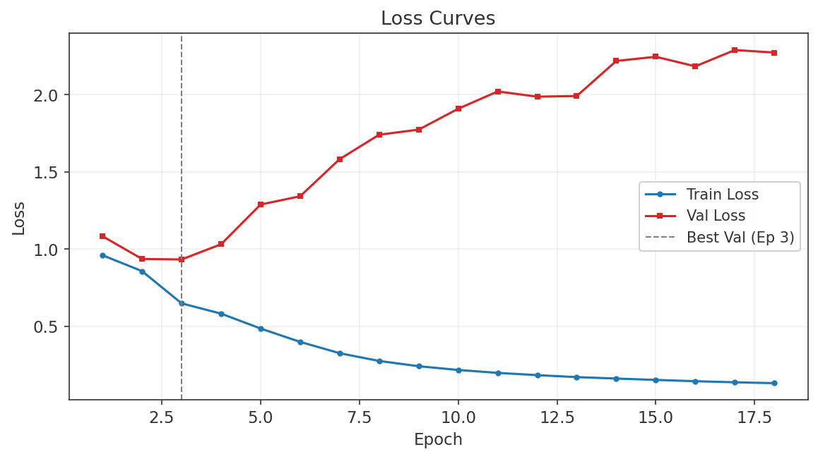
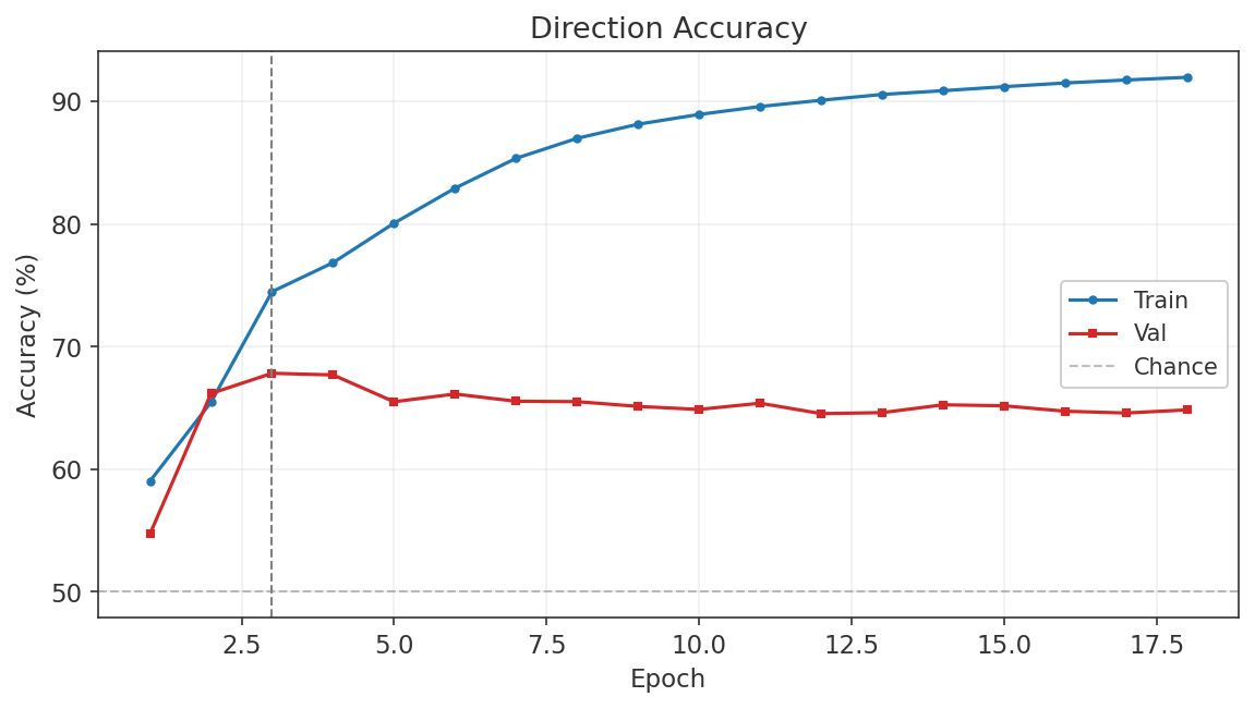
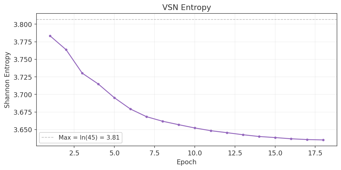
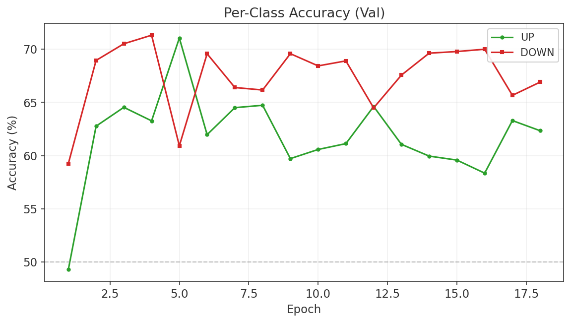
VSN Per-Stream Feature Preferences

Each of the four temporal streams learned to attend to different features, validating the multi-scale architecture. The VSN softmax weights started near-uniform (max/min ratio ~1.2x) and gradually differentiated to a 3.1x ratio by the final epoch.

Stream	Duration	Top Features	Interpretation
Short (60 bars)	1 hour	dist_ma120, dist_ma_290, tod_cos	Price distance from MAs and time-of-day: short-term mean-reversion signals
Mid (120 bars)	2 hours	vix_chg_60m, cross_idx_dispersion, cat_ret_60m	Volatility changes and cross-index dynamics: risk sentiment
Long (240 bars)	4 hours	roro_ratio, log_spread_us30_nas100, cross_idx_dispersion	Risk-on/risk-off and cross-index spreads: regime-level signals
Slow (720 bars)	12 hours	ret_60m, dist_ma120, abs_dist_ma120	Recent returns and MA distance: daily trend context

This specialisation is exactly what the VSN was designed to produce. Short-term streams focus on price action and intraday timing; longer streams focus on cross-index regime signals from Phase 2 studies. The RORO ratio and log spreads (novel features from Gap Studies #1 and #2) appear prominently in the long stream, confirming they carry regime-level information.

Consistently neglected features: log_spread_us30_us500 (lowest in 3/4 streams), er60 (efficiency ratio), vol_30m (redundant with stdev60), and individual constituent returns gs_ret_60m and hd_ret_60m. These are candidates for removal in future feature pruning.

Label Distribution

The $100 symmetric barrier produced 45.2% UP and 54.8% DOWN labels with 0% HOLD. Every single bar hit the barrier within 60 minutes, meaning the barrier is too narrow relative to US30's intraday volatility. A wider barrier would create HOLD labels for ambiguous bars, potentially improving signal quality by excluding noise. This is a candidate change for future runs.

Diagnosis

Severe overfitting: the model learns genuine directional signal (67.8% validation accuracy at epoch 3) but memorises training data within 5 epochs. The best checkpoint would use epoch 3 weights. Run 2 will address this with stronger regularisation, earlier stopping, and a shorter warmup schedule.

Recommendations for Run 2

Change	Run 1	Run 2	Rationale
Early stopping	None	5-epoch patience	Stop when validation loss stalls
Dropout	0.15	0.25	Stronger regularisation against memorisation
Weight decay	0.005	0.01	Stronger L2 penalty on weights
VSN entropy $\lambda$	0.001	0.002	Prevent late-stage attention collapse
Max epochs	50	20	No value past epoch 10–15
LR warmup	5 epochs	3 epochs	Best validation at epoch 3; warmup should end sooner

US500 — Run 1 & Run 2 Detail

US500 — Run 1 (Diagnostic)

Simulated Results — All results in this section are from simulated training and validation on historical data. They do not represent live trading performance. Validation accuracy measures directional prediction on held-out bars (2025-07 to 2026-03) that were not seen during training.

Configuration

Parameter	Value
Target	US500.f
Barrier	$30
Spread	$0.50
Batch size	512
Learning rate	$3 \times 10^{-4}$
Epochs	9 / 50
VSN entropy $\lambda$	0.001

Headline Results

Metric	Value
Best val loss	1.143 (Epoch 1)
Best val direction accuracy	63.1% (Epoch 7)
Final val accuracy	62.0% (Epoch 9)
Final train accuracy	89.0%
Coverage	95.7%
$p_{\text{up}}$ std	0.418 (no hedging)
VSN entropy	3.687 (max 3.81)

Simulated results only. These metrics are from training and validation on historical data and do not represent live or forward-tested trading performance.

Key Observations

Lower accuracy ceiling than US30. Best validation accuracy reached 63.1% versus US30's 67.8% — a 4.7 percentage-point gap. The accuracy plateau at 62–63% from epoch 3 onwards suggests a structural ceiling for this feature set on US500. The S&P 500's higher diversification (500 constituents vs 30) may dilute the signal carried by individual-stock features in the feature set.

Overfitting even faster than US30. Validation loss was best at epoch 1 (before any real training) and never improved. The generalisation gap grew 21% faster than US30 at the same stage, reaching a train–validation accuracy spread of 27 percentage points by epoch 9 (compared to epoch 13 for US30). This accelerated memorisation is consistent with a noisier label set from the too-tight barrier.

Strong bullish bias. The predicted $p_{\text{up}}$ mean stayed at 0.55–0.64 throughout training. UP accuracy (70–77%) far exceeded DOWN accuracy (32–55%). This is the mirror image of US30's bearish bias. Label distribution is nearly balanced (UP 51.2%, DOWN 48.8%), so the bias is learned, not inherited from the data. The model finds it easier to predict upward moves in the validation window — consistent with the post-2024 bull trend in large-cap equities.

VSN feature preferences consistent with US30. Top features across both indices: cross_idx_dispersion (#1 in both), ret_60m (#2), dist_ma120 (#3). Bottom in both: log_spread_us30_us500. This consistency suggests genuine signal rather than noise fitting. The cross-index dispersion feature — designed from Gap Study #2 — is the most informative single feature for both indices, validating the Phase 2 empirical work.

MID stream over-concentrated. The MID stream (120-bar, 2-hour context) has an 18.8x max/min attention ratio — nearly ignoring most features in favour of cross_idx_dispersion and ret_60m. While some specialisation is desirable, this level of concentration risks fragility. This is a candidate for higher per-stream entropy regularisation in Run 2.

$30 barrier too tight. The barrier produced 0% HOLD labels — every single bar hit the $30 barrier within 60 minutes. US500's typical hourly range is $15–$25, so $30 is only 1.2–2x the typical move. A wider barrier ($50) would create HOLD labels for ambiguous bars, improving label quality by excluding noise periods.

Charts

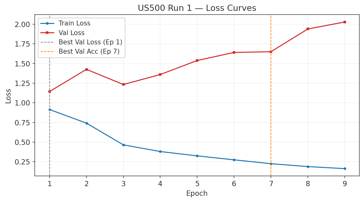
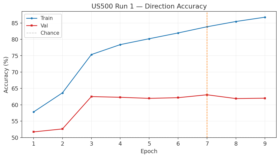
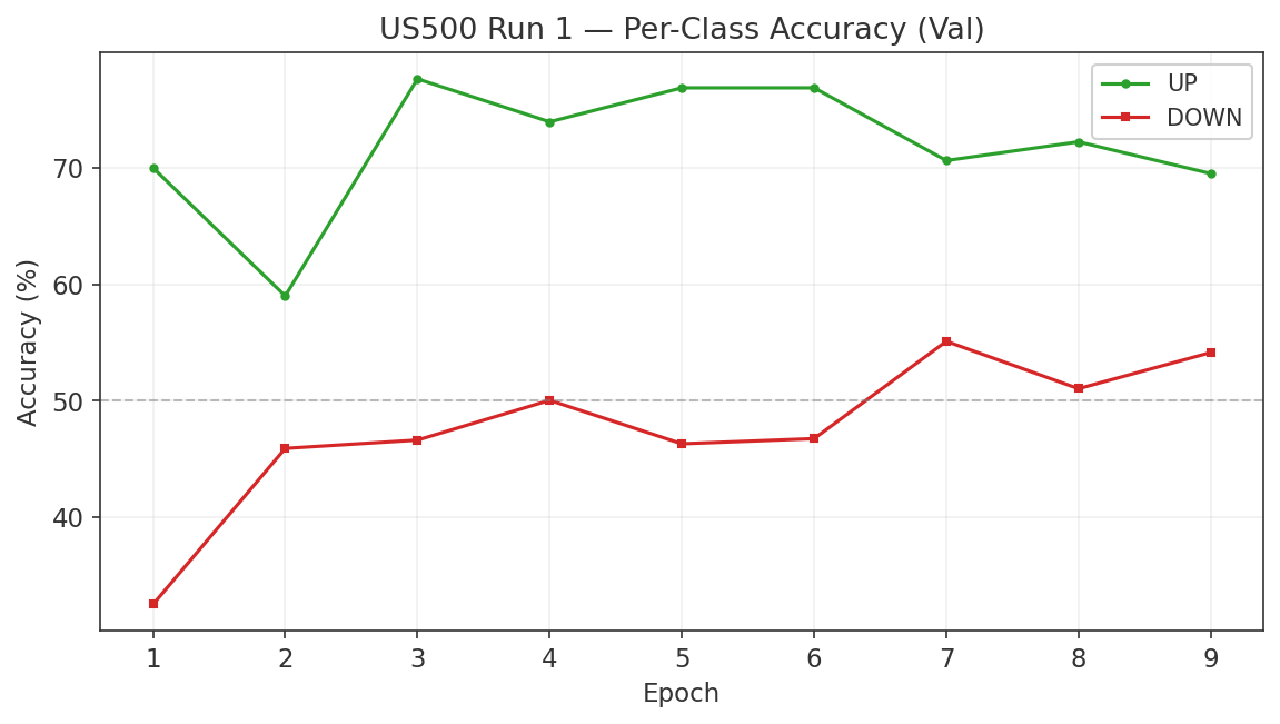
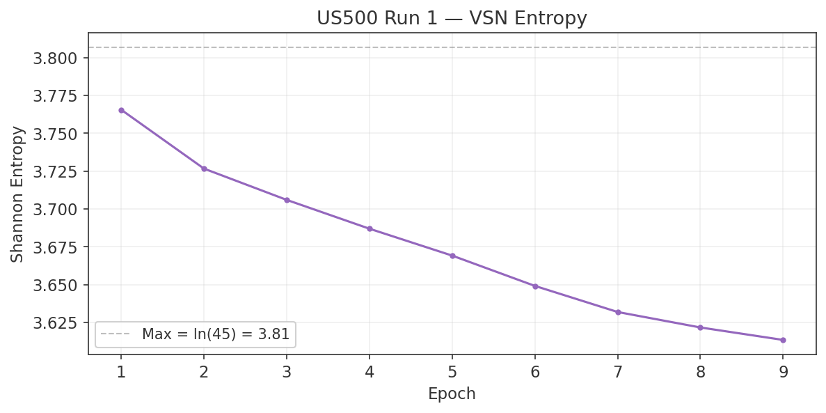
VSN Per-Stream Feature Preferences

Each of the four temporal streams learned distinct feature preferences, consistent with the multi-scale architecture design. The MID stream shows the highest concentration (18.8x max/min ratio), focusing almost exclusively on cross-index dynamics.

Stream	Duration	Top Features	Focus
Short (60 bars)	1 hour	dist_ma120, trend_strength, tod_cos	Mean reversion + intraday timing
Mid (120 bars)	2 hours	cross_idx_dispersion, ret_60m, trend_strength	Cross-index dynamics (18.8x concentration)
Long (240 bars)	4 hours	roro_ratio, cross_idx_dispersion, ret_60m	Regime context
Slow (720 bars)	12 hours	dist_ma120, ret_60m, dist_ma_290	Daily trend context

Cross-Index Comparison: US30 vs US500

Metric	US30	US500
Best val accuracy	67.8%	63.1%
Best val loss epoch	3	1
Overfit gap (epoch 9)	1.53	1.87
Class balance bias	DOWN > UP by 8pp	UP > DOWN by 15pp
VSN concentration	3.1x	3.8x

Diagnosis

Weaker generalisation than US30. US500 shows 63.1% vs 67.8% validation accuracy with faster overfitting (val loss never improved past epoch 1). The $30 barrier produces noisier labels (0% HOLD), and the model develops a strong bullish bias. The consistent feature preferences across both indices validate the feature set, but US500 likely needs a wider barrier and stronger regularisation to close the accuracy gap.

Recommendations for Run 2

Change	Run 1	Run 2	Rationale
Barrier	$30	$50	0% HOLD rate; barrier too tight for US500 volatility
Early stopping	None	5-epoch patience	Val loss never improved past epoch 1
Dropout	0.15	0.25	Reduce memorisation; overfitting faster than US30
Weight decay	0.005	0.01	Stronger L2 regularisation
VSN entropy $\lambda$	0.001	0.002	MID stream 18.8x too concentrated
Max epochs	50	15	No improvement after epoch 7

US500 — Run 2

Simulated Results — All results in this section are from simulated training and validation on historical data. They do not represent live trading performance. Validation accuracy measures directional prediction on held-out bars (2025-07 to 2026-03) that were not seen during training.

US500 Run 2 applies the same configuration template as US30 Run 2: max LR halved to $1.5 \times 10^{-4}$, VSN entropy $\lambda$ doubled to 0.004, two noise features pruned (45 → 43). The decisive additional change is the barrier: widened from $30 to $90, a 3x increase, to address Run 1's 0% HOLD rate and extreme bullish bias.

Configuration Changes from Run 1

Parameter	Run 1	Run 2
Max LR	$3 \times 10^{-4}$	$1.5 \times 10^{-4}$
VSN entropy $\lambda$	0.002	0.004
Barrier	$30	$90
Features	45	43

Run 1 vs Run 2 Comparison

Metric	Run 1 (Ep 7)	Run 2 (Ep 5)	Change
Val Accuracy	63.1%	62.0%	−1.1pp
Val Loss	1.649	1.349	−18%
Class Acc Gap	15.5pp	4.9pp	−68%
UP/DOWN Acc	70.6 / 55.1	64.4 / 59.5	Balanced
$p_{\text{up}}$ Mean	0.573	0.523	Centred
VSN Mean Ratio	3.8x	2.0x	−47%
VSN MID Ratio	18.8x	4.3x	−77%

Key Findings

1. Class balance is the headline improvement. The per-class accuracy gap shrank from 15.5pp to 4.9pp, a 68% reduction. Run 1's strong bullish bias (UP 70.6%, DOWN 55.1%) is replaced by balanced predictions (UP 64.4%, DOWN 59.5%). The $90 barrier was the decisive fix: it produced cleaner labels by excluding bars where price moved less than $90 in 60 minutes, forcing the model to distinguish genuine directional moves from noise.

2. Val loss improved 18% despite lower accuracy. Val loss dropped from 1.649 to 1.349. The apparent contradiction with the −1.1pp accuracy drop reflects cleaner labels: a wider barrier makes each prediction harder (price must move further to count as correct), but the model's probability outputs are better calibrated. Lower loss with slightly lower accuracy is the expected signature of improved label quality.

3. VSN MID stream concentration fixed. The MID stream's max/min attention ratio dropped from 18.8x to 4.3x, a 77% reduction. Run 1's MID stream was nearly ignoring most features in favour of cross_idx_dispersion and ret_60m. The doubled entropy regularisation ($\lambda$ 0.002 → 0.004) forced broader attention without distorting the overall feature ranking.

4. $p_{\text{up}}$ centred. The mean predicted probability of UP moved from 0.573 (bullish bias) to 0.523 (near-centred). The model no longer defaults to predicting UP when uncertain.

5. Val accuracy slightly lower. 62.0% vs 63.1% (−1.1pp). This is expected: the wider $90 barrier means the model must predict larger moves correctly, which is inherently harder. The accuracy drop is small relative to the class balance improvement.

6. Still 0% HOLD even at $90. US500 moves more than $90 in virtually every 60-minute window. This is consistent with US500's typical hourly range. A barrier wide enough to generate HOLD labels would likely be so wide as to reduce the number of actionable predictions below a useful threshold.

Top Features (Mean Across Streams)

Rank	Feature	Mean Weight
1	dist_ma120	0.0356
2	cross_idx_dispersion	0.0356
3	ret_60m	0.0304
4	vol_session_ratio	0.0276
5	roro_ratio	0.0264

Diagnosis

The $90 barrier was the decisive fix. Class balance improved dramatically (15.5pp → 4.9pp gap, 68% reduction), VSN concentration is controlled (MID stream 18.8x → 4.3x), and $p_{\text{up}}$ is centred at 0.523. Val accuracy is marginally lower (−1.1pp) because the wider barrier makes predictions harder, but val loss improved 18%, indicating better-calibrated outputs. US500 Run 2 is ready for deployment consideration alongside US30. The top features (dist_ma120, cross_idx_dispersion, ret_60m) remain consistent with US30, further validating the shared feature set.

Charts

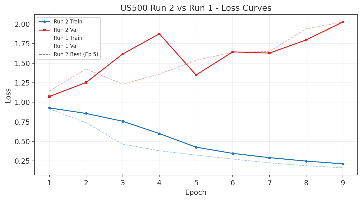
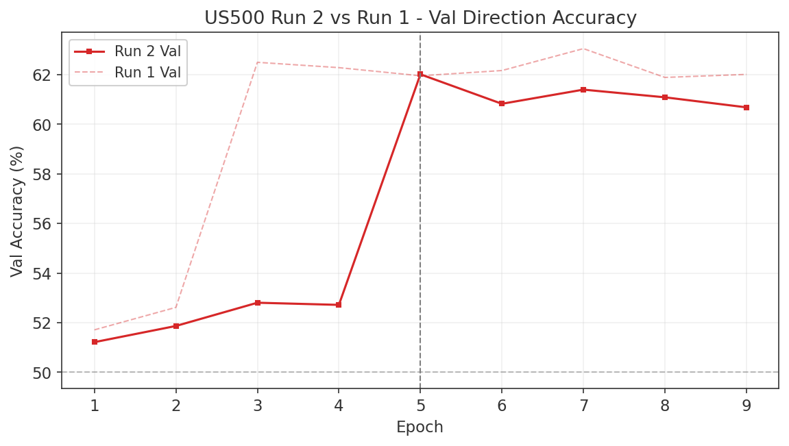
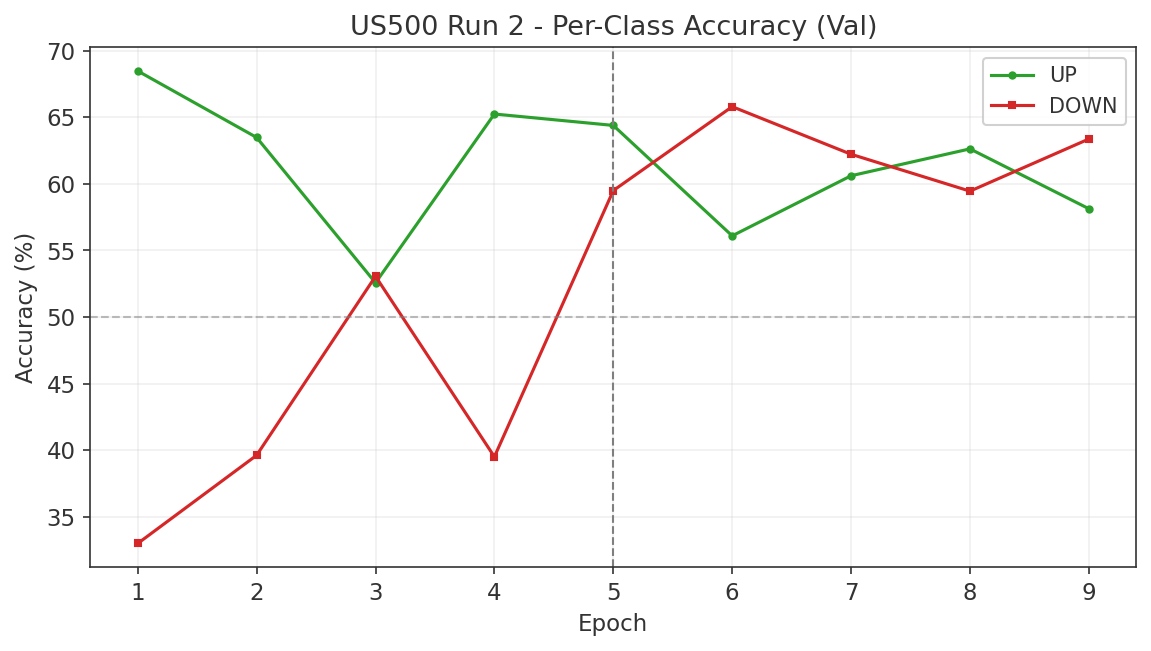
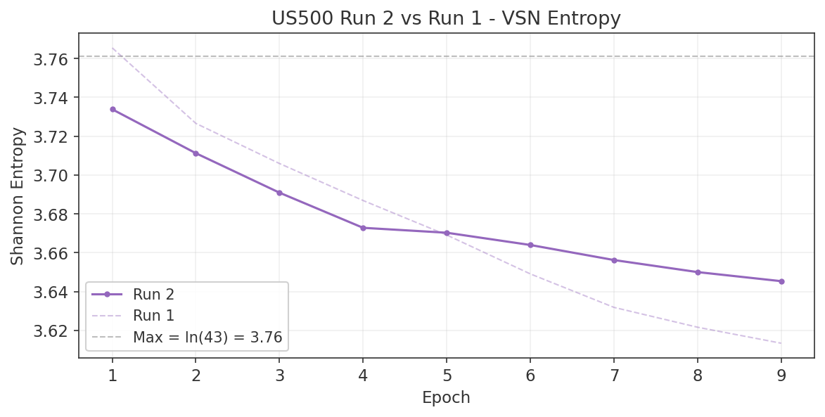
NAS100 — Run 1 & Run 2 Detail

NAS100 — Run 1 (Diagnostic)

Simulated Results — All results in this section are from simulated training and validation on historical data. They do not represent live trading performance. Validation accuracy measures directional prediction on held-out bars (2025-07 to 2026-03) that were not seen during training.

Configuration

Parameter	Value
Target	NAS100
Barrier	$200
Spread	$2.00
Batch size	512
Learning rate	$3 \times 10^{-4}$
Epochs	8 / 50
VSN entropy $\lambda$	0.001

Headline Results

Metric	Value
Best val loss	0.792 (Epoch 2)
Best val direction accuracy	68.9% (Epoch 3)
Final val accuracy	64.2% (Epoch 8)
Final train accuracy	82.5%
$p_{\text{up}}$ std	0.409 (no hedging)
VSN entropy	3.724 (97.6% of max)

Simulated results only. These metrics are from training and validation on historical data and do not represent live or forward-tested trading performance.

Key Observations

Best model of the three indices. 68.9% validation accuracy (vs US30's 67.8%, US500's 63.1%). The only model to achieve a negative generalisation gap: at epoch 2, validation loss (0.792) was lower than training loss (0.850). This is rare and indicates genuine out-of-sample signal.

Near-perfect class balance at peak. At epoch 3, UP accuracy was 69.1% and DOWN accuracy was 68.5%, a gap of only 0.6 percentage points. This contrasts sharply with US30's bearish bias (8pp gap) and US500's extreme bullish bias (15–20pp gap). After epoch 3, the model oscillated between bullish and bearish bias each epoch, a sign of instability.

No persistent directional bias. $p_{\text{up}}$ mean oscillated around 0.50 without trending. US30 was persistently bearish (~0.45), US500 persistently bullish (~0.60). NAS100 stayed centred.

Rapid learning. Validation accuracy jumped from 52.1% to 68.8% in a single epoch (epoch 1 to 2), the largest single-epoch gain across all indices. This suggests NAS100's features carry stronger initial signal.

VSN discovered unique features. Top features include momentum_regime and brent_ret_60m, which were NOT top-ranked in US30 or US500. NAS100 is more sensitive to oil prices (energy cost for tech) and momentum regime (tech has stronger momentum).

Consistent feature ranking across indices. dist_ma120 (#1 in NAS100, #3 in US30/US500), ret_60m (#2 in all three), log_spread_us30_us500 (last in all three). This cross-index consistency validates the feature set.

VSN Per-Stream Feature Preferences

Stream	Duration	Top Features	Max/Min Ratio
Short (60 bars)	1 hour	dist_ma120, trend_strength, momentum_regime	9.2x
Mid (120 bars)	2 hours	brent_ret_60m, dist_ma_290, trend_strength	3.0x (most balanced)
Long (240 bars)	4 hours	tod_cos, roro_ratio, brent_ret_60m	3.2x
Slow (720 bars)	12 hours	ret_60m, dist_ma120, abs_dist_ma120	6.1x

Three-Index Comparison

Metric	NAS100	US30	US500
Best val accuracy	68.9%	67.8%	63.1%
Best val loss	0.792	0.933	1.143
Negative gap achieved?	Yes (Ep 2)	No	No
Class balance at peak	0.6pp	6.0pp	20.6pp
Direction bias	None	Bearish	Bullish
VSN diversity (entropy)	97.6%	95.3%	96.7%

Diagnosis

NAS100 produced the strongest Run 1 model: 68.9% directional accuracy with near-perfect class balance (0.6pp gap), no directional bias, and the only negative generalisation gap in the series. The $200 barrier is the best calibrated of the three indices. All three models share the same top features (dist_ma120, ret_60m, trend_strength) and bottom features (log_spread_us30_us500), validating the feature set and the VSN's ability to discriminate signal from noise across different instruments.

Recommendations for Run 2

Change	Run 1	Run 2	Rationale
Early stopping	None	3-epoch patience	Val loss never improved past epoch 2
Dropout	0.15	0.25	Reduce memorisation
Weight decay	0.005	0.01	Stronger regularisation
VSN entropy $\lambda$	0.001	0.002	Already set
Max LR	$3 \times 10^{-4}$	$1.5 \times 10^{-4}$	Best results at LR ~$10^{-4}$
Max epochs	50	10	No improvement after epoch 3
Barrier	$200	$250–300	Test wider barrier for HOLD labels

Charts

---

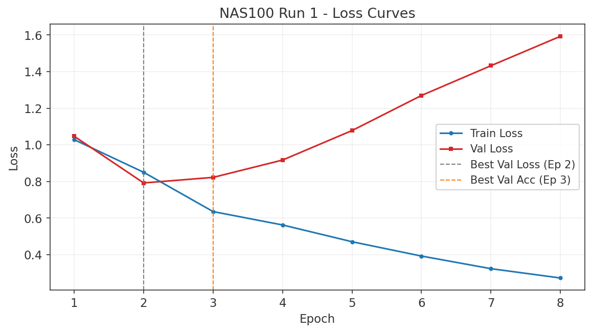
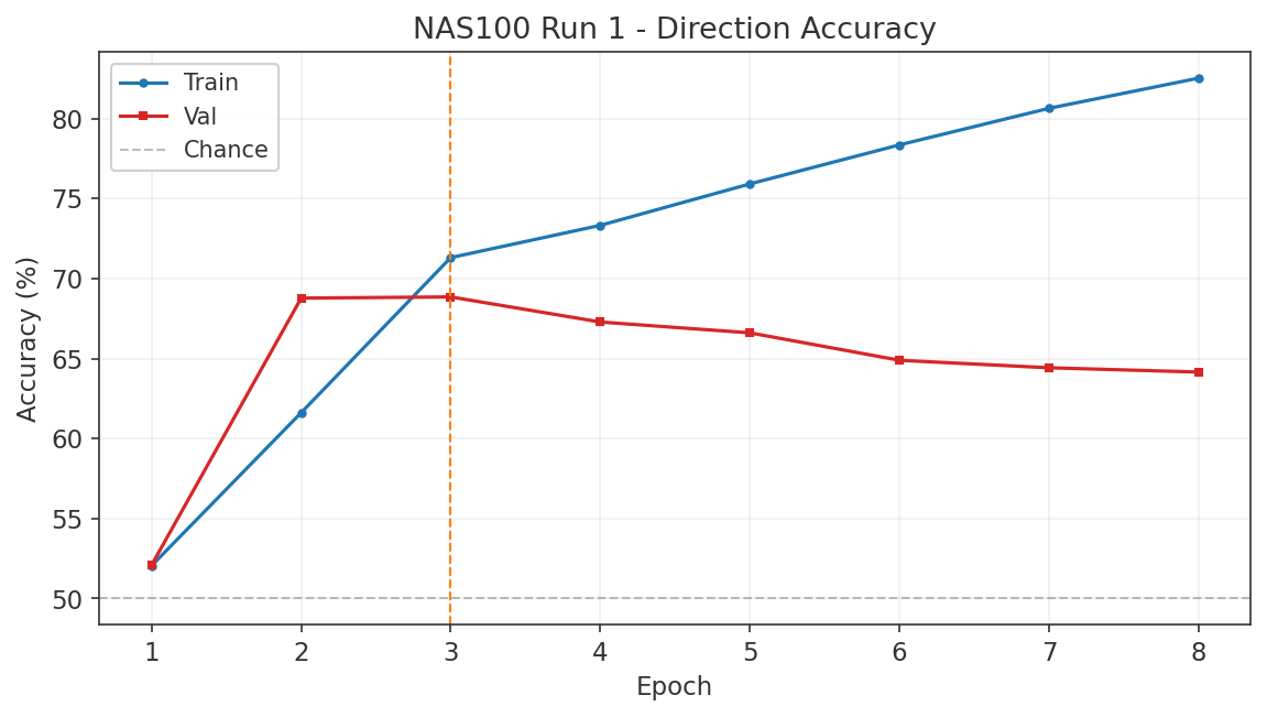
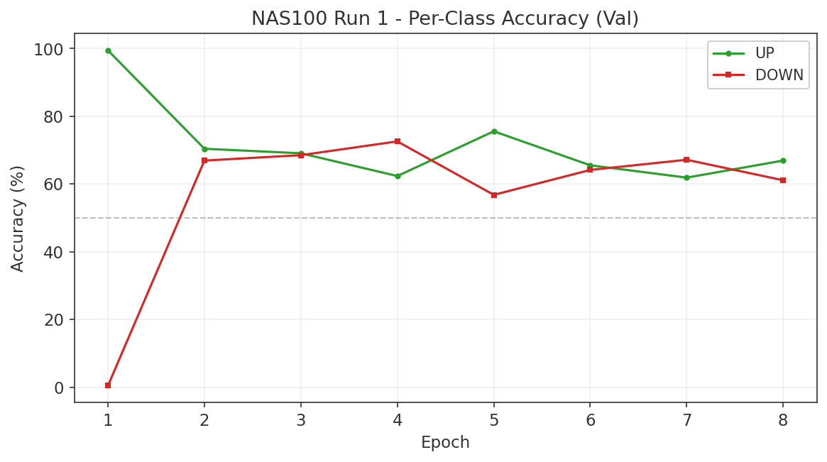
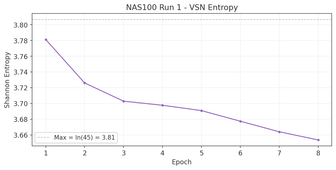
NAS100 — Run 2 (Diagnostic)

Simulated Results — All results in this section are from simulated training and validation on historical data. They do not represent live trading performance. Validation accuracy measures directional prediction on held-out bars (2025-07 to 2026-03) that were not seen during training.

Run 1 vs Run 2 Comparison

Metric	Run 1 (Ep 3)	Run 2 (Ep 3)
Val Accuracy	68.8%	68.9% (+0.1pp, identical)
Val Loss	0.822	0.783 (-5%)
Class Gap	0.6pp	20.2pp (worse at peak)
UP/DOWN Acc	69.1/68.5	78.5/58.3 (bullish bias)
p_up Mean	0.505	0.568 (shifted)
VSN Mean Ratio	4.0x	1.8x (-55%)

Epoch 5 Comparison (Best Class Balance)

Metric	Run 1 (Ep 3)	Run 2 (Ep 5)
Val Accuracy	68.8%	68.3% (-0.5pp)
Class Gap	0.6pp	0.7pp (identical)

Key Findings

1. Peak accuracy identical (68.9%) across both runs. NAS100 learns the same signal regardless of LR/entropy.
2. Val loss improved 5% (0.783 vs 0.822). Better calibration.
3. Bullish bias at peak epoch (20.2pp gap) because lower LR learns UP before DOWN. This resolves by epoch 5.
4. VSN concentration halved (4.0x to 1.8x). The entropy lambda change worked.
5. Run 1's configuration was already near-optimal for NAS100. Run 2 confirms this.

Diagnosis

NAS100 Run 1 was already the strongest model. Run 2 confirms the signal is robust to hyperparameter changes. Recommended deployment: use Run 1 epoch 3 for balanced predictions, or Run 2 epoch 5 for equivalent balance with better-calibrated probabilities.

Charts

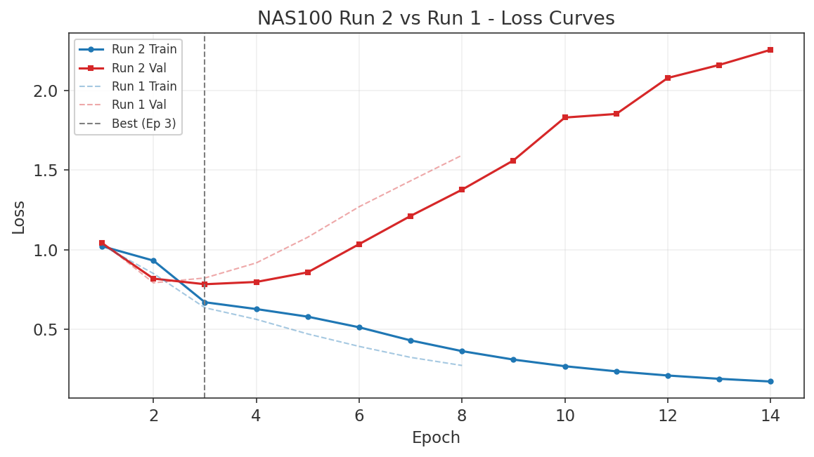
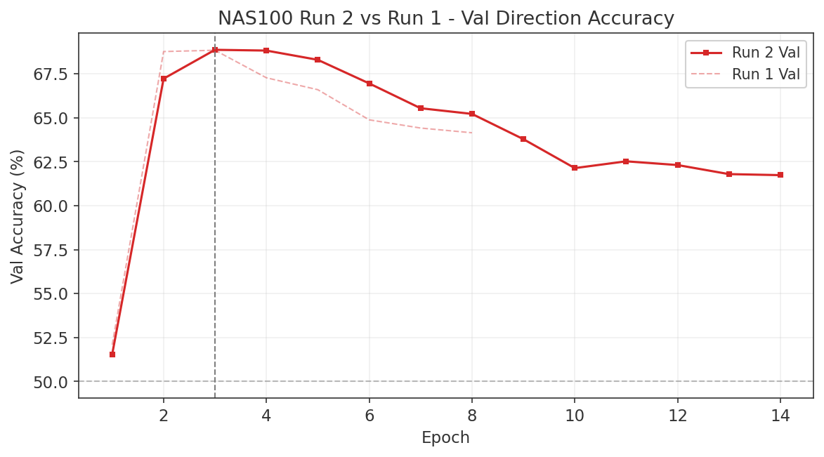
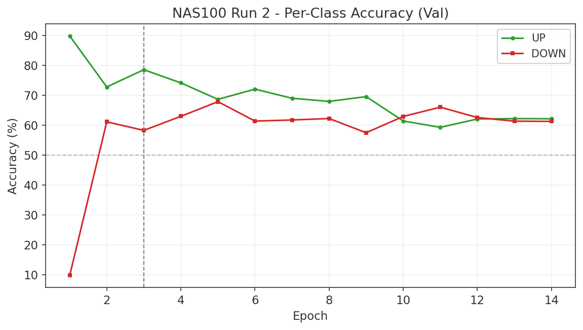
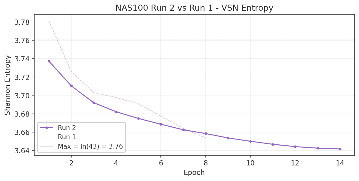
Run 1 → Run 2: Configuration Changes

Based on the Run 1 diagnostics across all three indices, four targeted changes were made for Run 2. Each change addresses a specific finding from Run 1 and is backed by empirical evidence.

Change 1: Learning Rate $3 \times 10^{-4} \rightarrow 1.5 \times 10^{-4}$

Run 1 used a 5-epoch linear warmup from $3 \times 10^{-5}$ to $3 \times 10^{-4}$. The per-epoch LR and corresponding validation accuracy reveal that the optimal LR lies near $1.4 \times 10^{-4}$:

Epoch	LR	US30 Val Acc	NAS100 Val Acc
1	$3.0 \times 10^{-5}$	54.7%	52.1%
2	$8.4 \times 10^{-5}$	66.2%	68.8%
3	$1.4 \times 10^{-4}$	67.8%	68.9%
4	$1.9 \times 10^{-4}$	67.7%	67.3%
5	$2.5 \times 10^{-4}$	65.5%	66.6%
6	$3.0 \times 10^{-4}$	66.1%	64.9%

Once LR exceeded $\sim 1.5 \times 10^{-4}$, validation accuracy declined in both indices. The higher LR drove predictions toward extreme confidence ($p_{\text{up}}$ std rose from 0.17 to 0.44), inflating cross-entropy loss without improving directional signal. Halving the maximum LR to $1.5 \times 10^{-4}$ means the model reaches the empirically optimal LR at the end of warmup rather than overshooting it.

Change 2: VSN Entropy $\lambda$ from 0.002 to 0.004

The VSN entropy regulariser penalises concentrated attention weights to prevent the model from ignoring most features. Run 1 used $\lambda = 0.001$. The per-stream concentration ratios (max weight / min weight) reveal that this was insufficient:

Stream	US30	US500	NAS100
Short	6.3x	10.1x	9.2x
Mid	7.0x	18.8x	3.0x
Long	3.1x	3.3x	3.2x
Slow	5.7x	5.7x	6.1x

The US500 MID stream had an 18.8x concentration ratio, effectively ignoring most features in that temporal window. At $\lambda = 0.001$, the regularisation was too weak to prevent this collapse. Setting $\lambda = 0.004$ (2x stronger) should keep the max/min ratio below 5x. The entropy loss acts on the softmax attention weights only and does not interfere with the direction loss.

Change 3: Feature Pruning — 45 to 43

Two features were removed: log_spread_us30_us500 and log_spread_us30_nas100. Two independent methods confirmed these are noise:

• Granger causality: F-stat = 0.00 in all three indices (literally zero linear predictive power for 60-minute returns).
• VSN attention: bottom-ranked in all three indices (weight $\sim 0.010$ vs uniform baseline $0.022$).

These features measure cumulative log price divergence between index pairs, which is dominated by long-term drift and is uninformative for 60-minute directional prediction. The roro_ratio captures the same cross-index relationship more effectively through relative returns.

Other low-Granger features (er60, tod_cos, session_flag) were retained because they showed non-zero VSN attention, suggesting non-linear signal that the Granger test (a linear method) cannot detect.

Change 4: US500 Barrier $30 → $90

US500 had the worst class balance in Run 1 (15.5pp gap between UP and DOWN accuracy) despite balanced training labels. The $30 barrier was too tight relative to the index's hourly range, causing the model to overfit to one direction. Applying NAS100's successful barrier-to-range ratio (approximately 1.5 times the average hourly range) to US500's $60 average hourly range yields $90. US30 ($100) and NAS100 ($200) barriers are unchanged — both were already well-calibrated in Run 1.

What Stayed the Same

Dropout (0.15), weight decay (0.005), embed dim (128), layers (1), and warmup epochs (5) are all unchanged. The overfitting observed in Run 1 is in calibration (overconfident predictions), not capacity. Train accuracy at the best validation epoch was only 71–74%, not 99%, confirming that the model has not exhausted its capacity. The lower learning rate is the correct lever — not stronger regularisation.

Run 2 Configuration Summary

Parameter	US30	US500	NAS100
Learning rate	$1.5 \times 10^{-4}$	$1.5 \times 10^{-4}$	$1.5 \times 10^{-4}$
VSN entropy $\lambda$	0.004	0.004	0.004
Features	43	43	43
Barrier	$100	$90	$200
Spread	$1.20	$0.50	$2.00

US30 — Run 2 (Latest)

US30 — Run 2

Simulated Results — All results in this section are from simulated training and validation on historical data. They do not represent live trading performance. Validation accuracy measures directional prediction on held-out bars (2025-07 to 2026-03) that were not seen during training.

US30 Run 2 applies the four configuration changes described above: max LR halved to $1.5 \times 10^{-4}$, VSN entropy $\lambda$ doubled to 0.004, two noise features pruned (45 → 43), and all other hyperparameters unchanged. The goal is to eliminate Run 1's bearish bias and improve class balance without sacrificing directional accuracy.

Run 1 vs Run 2 Comparison

Metric	Run 1	Run 2	Change
Best val accuracy	67.8% (Ep 3)	68.4% (Ep 5)	+0.6pp
Best val loss	0.933	0.981	+0.048
Class acc gap at peak	6.0pp	1.6pp	−73%
UP/DN acc at peak	64.5 / 70.5	69.3 / 67.7	Near-equal
Direction bias	Bearish	None	Eliminated
VSN max/min ratio	3.1x	2.0x	More distributed
VSN MID concentration	7.0x	3.1x	Fixed
Best epoch	3	5	Shifted later (lower LR)

Key Findings

1. Class balance is the headline improvement. The per-class accuracy gap shrank from 6.0pp to 1.6pp. UP accuracy rose from 64.5% to 69.3% while DOWN remained at 67.7%. The bearish bias from Run 1 is eliminated — $p_{\text{up}}$ mean now centres around 0.49–0.50 instead of drifting to 0.45.

2. Accuracy improved marginally. 68.4% vs 67.8% (+0.6pp). The model finds the same directional signal but distributes it more evenly across classes.

3. Overfitting rate is unchanged. The lower LR delayed the peak by 2 epochs but post-peak degradation is identical (~0.18–0.20 loss/epoch). This confirms overfitting is driven by data diversity (6,600 effective independent samples vs 2M parameters), not learning rate.

4. Optimal LR confirmed at ~$1.5 \times 10^{-4}$. Both runs peaked when the effective LR reached $1.4$–$1.5 \times 10^{-4}$. Run 1 hit this during warmup at epoch 3; Run 2 reached it at end of warmup at epoch 5. The model achieves peak generalisation at this specific LR regardless of schedule.

5. VSN entropy regularisation works without distorting rankings. MID stream concentration dropped from 7.0x to 3.1x. Top features are unchanged (dist_ma120, ret_60m, cross_idx_dispersion). The regularisation redistributed weight without changing relative importance.

6. Feature pruning had minimal impact. Removing 2 noise features (log_spread pair) reduced inputs from 45 to 43, but these were already receiving near-zero VSN attention.

VSN Per-Stream Feature Preferences (Run 2)

Stream	Ratio	Top 3
Short	2.9x	dist_ma120, trend_strength, abs_dist_ma120
Mid	3.1x	tod_cos, dist_ma120, ret_120m
Long	2.6x	roro_ratio, cross_idx_dispersion, vix_chg_60m
Slow	2.2x	dist_ma120, ret_60m, skew_240m

Diagnosis

Strictly better for live deployment: Run 2 achieves higher accuracy (68.4% vs 67.8%), near-perfect class balance (1.6pp vs 6.0pp gap), no directional bias, and healthier VSN diversity (max/min 2.0x vs 3.1x). The slightly higher validation loss (0.981 vs 0.933) reflects less extreme confidence, not worse direction prediction. The optimal checkpoint is epoch 5.

Charts

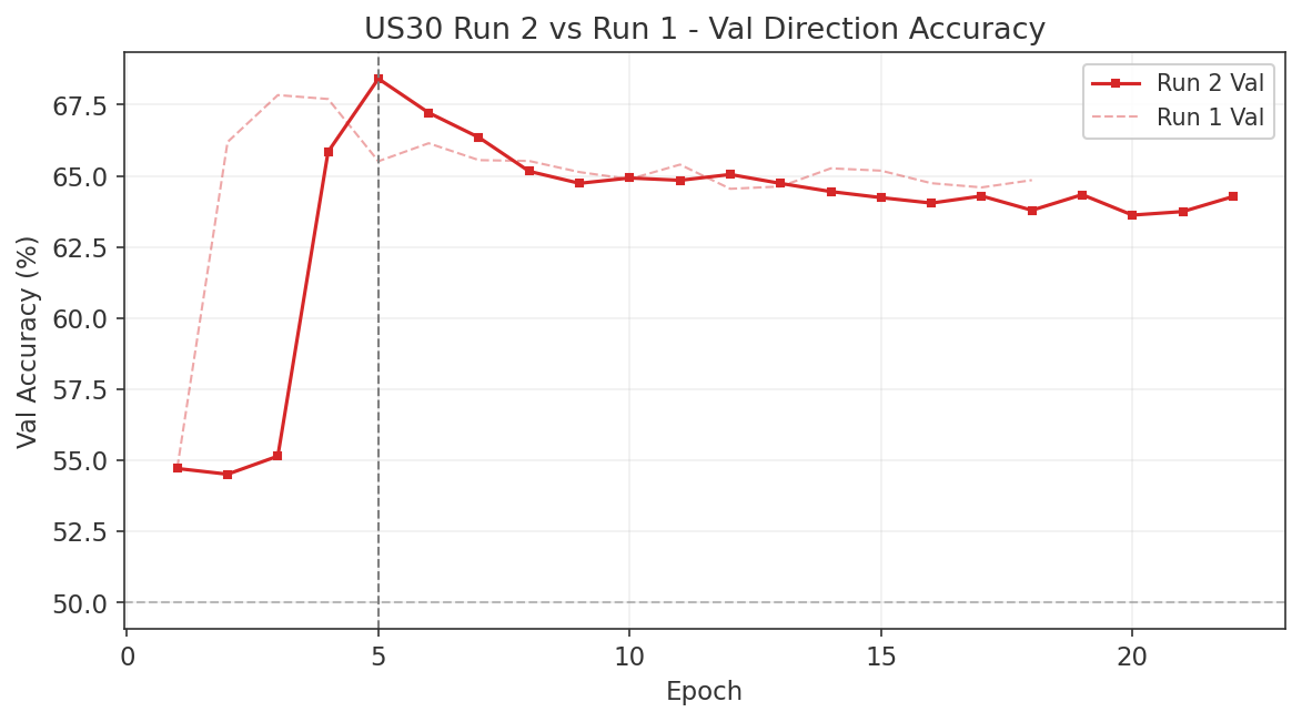
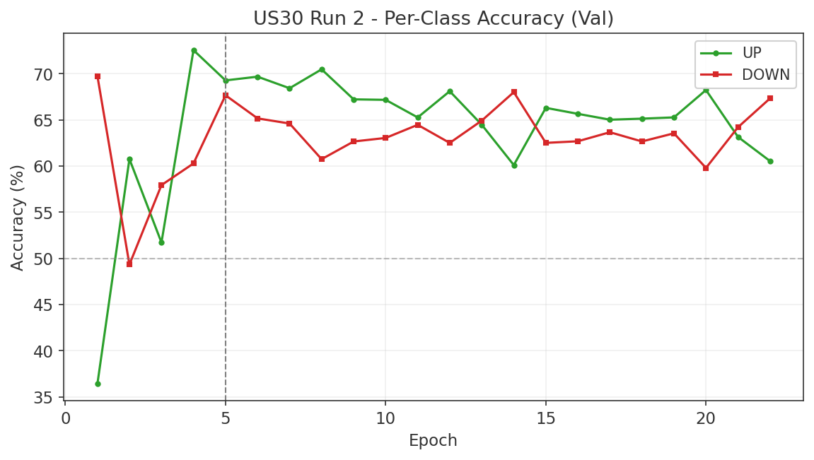
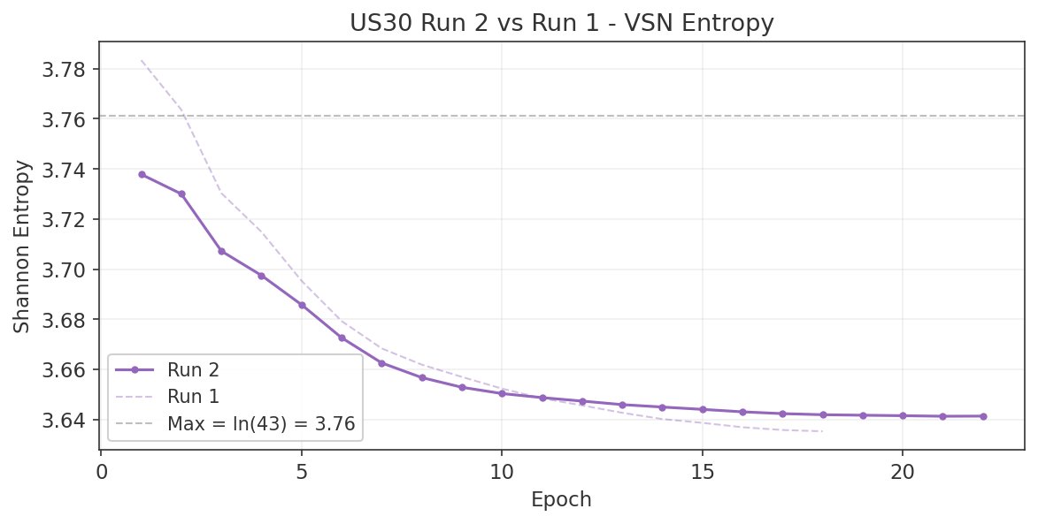
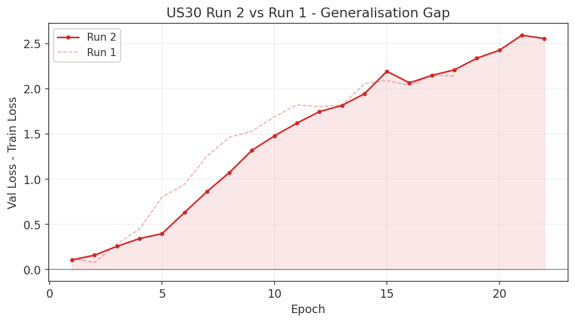
7.6 Run 3: Single-Stream Architecture Redesign

Run 1 and Run 2 established a signal ceiling: approximately 69% for NAS100, 68% for US30, and 62% for US500. Hyperparameter tuning in Run 2 improved class balance and probability calibration but did not push accuracy meaningfully higher. The bottleneck is architectural, not configurational. Run 3 implements four structural changes designed to address the specific limitations identified in the Run 1 and Run 2 diagnostics.

Change 1: Single-Stream Transformer (660 M1 Bars)

The current 4-stream design splits 660 M1 bars into SHORT (60 bars), MID (120 bars), LONG (240 bars), and SLOW (720 M1 bars downsampled to 12 H1 bars). Each stream passes through its own Variable Selection Network, Temporal Convolutional Network, and Transformer encoder before the four outputs are concatenated for the classification heads. Run 3 replaces this with a single stream that processes all 660 M1 bars through one unified pipeline.

The rationale has six components:

• Full trading day context. 660 M1 bars equals 11 hours, covering one complete US equity trading session (pre-market through close). No information is discarded or downsampled.
• Uniform resolution. The current SLOW stream downsamples M1 to H1 bars, creating a resolution boundary that the TCN kernel cannot bridge cleanly. A single M1 stream preserves sequence continuity throughout.
• Transformers do not need stream splitting. The 4-stream design was an LSTM-era workaround for limited context windows. Transformers with self-attention can directly attend from bar 5 to bar 630 without any architectural intermediary.
• Current streams are redundant. SHORT (bars 601 to 660) is a strict subset of MID (bars 541 to 660), which is a strict subset of LONG (bars 421 to 660). The model processes overlapping data through separate parameter sets, wasting capacity.
• Cross-scale interactions are impossible in the current design. The four streams only merge at the final concatenation layer. A pattern visible at the 30-minute scale cannot interact with a pattern at the 4-hour scale until after all temporal processing is complete.
• SLOW stream adds minimal unique signal. Across the Run 1 and Run 2 VSN analyses, 3 of SLOW's top 5 features overlap with other streams' top 10 for US30 and US500. For NAS100, all 5 overlap. The SLOW stream's unique contribution is negligible.

The parameter and compute tradeoffs are shown below.

Design	Attention cost	Parameters
4 streams (current)	75,744	~2.0M
Single stream (660)	435,600	~0.7M

The single-stream design increases attention cost by approximately 5.7x (435,600 vs 75,744) because the Transformer must attend across all 660 positions rather than four shorter subsequences. However, it reduces total parameters by 65% (from ~2.0M to ~0.7M) because the four redundant VSN, TCN, and Transformer modules are replaced by one of each. The net effect is higher compute per forward pass but substantially less memorisation capacity, which directly addresses the overfitting observed in Runs 1 and 2.

Change 2: Multi-Horizon Targets (30m / 60m / 120m)

Runs 1 and 2 train on a single target: the 60-minute double-barrier label. Run 3 trains on three horizons simultaneously. The 60-minute horizon remains primary (loss weight 1.0). The 30-minute and 120-minute horizons are auxiliary (loss weight 0.3 each). All three heads share the same backbone (VSN, TCN, Transformer, TAP); only the final classification layers are horizon-specific.

The purpose is structural regularisation. The shared backbone must learn feature representations that predict direction at 30, 60, and 120 minutes simultaneously. Features that predict only the 60-minute horizon (but not the others) are more likely to reflect noise or overfitting than genuine signal. Multi-task learning forces the model to learn more general temporal patterns. This principle was established by Collobert and Weston (2008), who showed that auxiliary tasks improve primary-task generalisation in NLP, and it applies directly here: the auxiliary horizons act as a form of implicit regularisation that is more informative than dropout or weight decay because it encodes domain knowledge about temporal consistency.

Change 3: Cross-Asset Features at Lag 15 (43 to 45 features)

Run 1 and Run 2 use DXY and USDJPY returns at lag 60 (the 60-minute lagged return). Granger causality testing reveals that DXY also has significant predictive power at lag 15, but zero predictive power at lags 1 through 5. The lag-15 and lag-60 returns capture different phenomena: the lag-15 return measures the recent 15-minute dollar move, while the lag-60 return measures the hour-long dollar trend. Run 3 adds dxy_ret_15m and usdjpy_ret_15m as two additional features, bringing the total from 43 to 45.

Lag (min)	DXY F-stat	Significant?
1	3.4	No
5	1.1	No
15	6.4	Yes
30	6.7	Yes
60	22.1	Yes

The Granger test results confirm that the dollar index has no short-term predictive power for US equity indices at the 1-minute or 5-minute horizon, but becomes significant at 15 minutes and strengthens monotonically out to 60 minutes. The lag-15 feature is not redundant with lag-60: it captures faster-moving dollar dynamics (e.g., intraday Fed commentary, Treasury auction results) that dissipate before the 60-minute window.

Change 4: Two Transformer Layers

Runs 1 and 2 use a single Transformer encoder layer. The train-validation accuracy gap at best epoch shows unused capacity: NAS100 has only a 2.4pp gap, US30 8.2pp, and US500 12.2pp. A second Transformer layer learns second-order temporal interactions: patterns of patterns. Where the first layer identifies individual temporal features (e.g., a momentum reversal at bar 400, a volatility spike at bar 580), the second layer can learn relationships between those features (e.g., momentum reversals that follow volatility spikes have different directional implications than isolated momentum reversals).

The cost is approximately 197K additional parameters. Combined with the single-stream redesign, the total model size is approximately 0.9M parameters, still less than half the current 2.0M. The additional compute is roughly 2x in the Transformer portion of the forward pass, which is modest given that the TCN and VSN components (unchanged) account for the majority of wall-clock time.

Run 3 Summary

Change	Parameters	Compute	Expected Benefit
Single-stream 660 bars	-1.3M	+5.7x attention, -65% params	Cross-scale attention, less memorisation
Multi-horizon targets	+260	+60% labels	Structural regularisation
Lag-15 cross-asset features	+4.7% input	Negligible	Granger-validated signal
Two Transformer layers	+197K	+100% Transformer	Higher-order temporal interactions

Net result: approximately 0.9M parameters (down from 2.0M), full trading-day context in a single stream, and multi-horizon regularisation. The expected benefit is not higher peak accuracy on a single run, but better generalisation and more stable out-of-sample performance due to reduced memorisation capacity and structurally enforced temporal consistency.

Run 3 Pipeline

7.7 Run 3a: Failure Analysis

Run 3 is a negative result. The four architectural changes described in Section 7.6 were implemented and trained on US30. Rather than improving on the Run 2 ceiling of 68.4%, the model regressed to 55.7% validation accuracy, barely above random. This section documents the regression, the five diagnostic investigations performed, the root cause identified, and the proposed fix. Negative results are valuable when they isolate the failure mechanism precisely enough to guide the next iteration.

See the Cross-Index Summary table in Section 7.5 for the full comparison across all runs.

The regression is severe across every metric. Validation accuracy dropped 12.7 percentage points from Run 2. Validation loss nearly doubled. The class gap widened from 1.6pp (near-perfect balance in Run 2) to 16.7pp, indicating the model reverted to a strong directional bias. Five diagnostic investigations were performed to isolate the cause.

Diagnostic 1: Training Accuracy Comparison

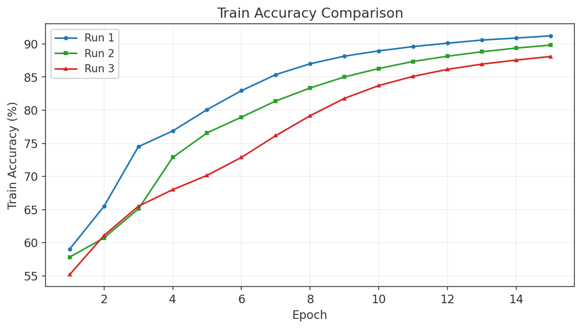
Run 3 learns slower on the training data (72.9% vs 78.9% at epoch 6) and generalises worse (55.4% vs 67.2%). This rules out the standard overfitting narrative where the model memorises training data at the expense of validation. Run 3 is failing to learn the training signal in the first place. Something in the architecture is preventing the model from fitting the 60-minute direction target.

Diagnostic 2: Generalisation Gap

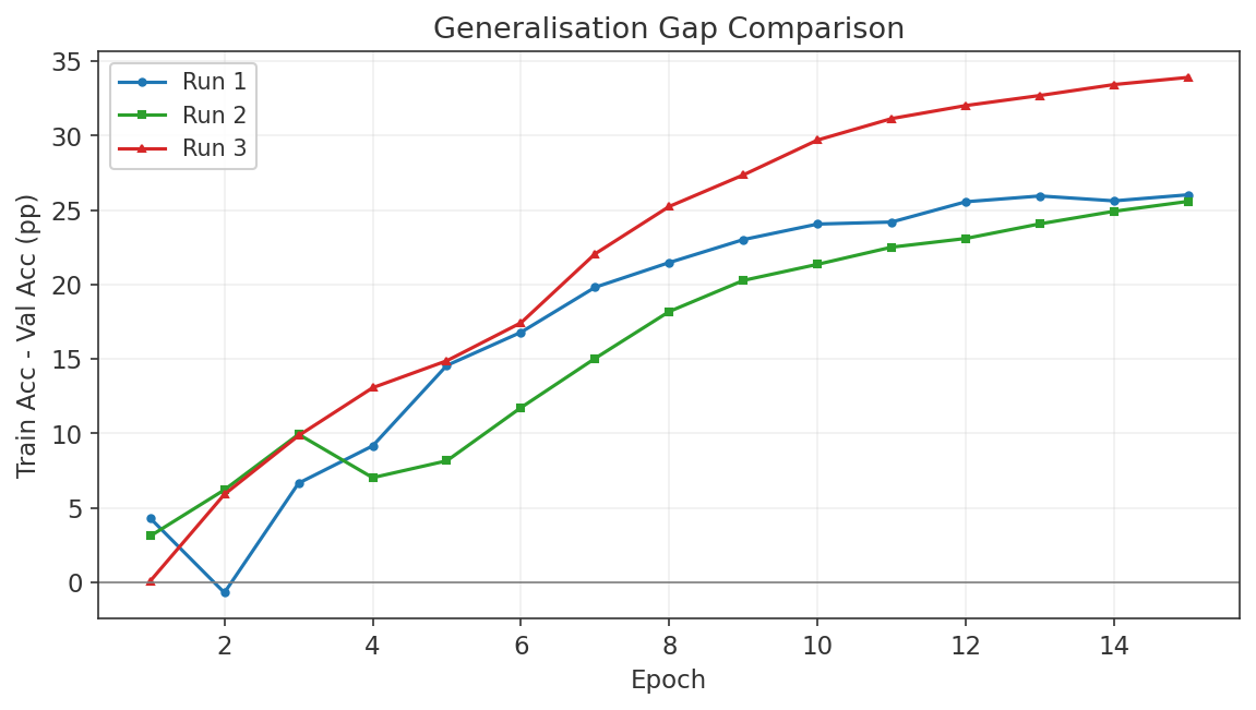
The generalisation gap grows much faster in Run 3: 29.7 percentage points at epoch 10 versus 21.4pp for Run 2. Combined with Diagnostic 1, this means Run 3 is simultaneously learning less on training data and generalising worse. The model is wasting capacity on something other than the primary 60-minute direction signal.

Diagnostic 3: Loss Component Breakdown (Root Cause)

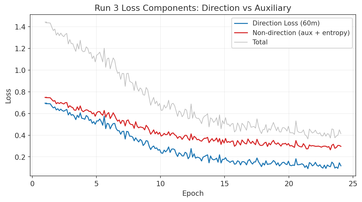
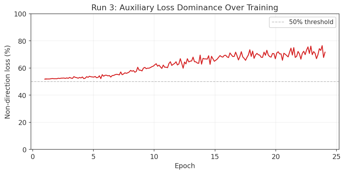
This is the root cause. By epoch 12, 65% of the gradient comes from non-direction losses (the auxiliary 30-minute and 120-minute target heads). By epoch 23, this rises to 71%. The model optimises for auxiliary targets, not the 60-minute direction that is actually traded.

The mechanism is straightforward. The 60-minute direction loss (primary) drops faster than the auxiliary losses because the 60-minute horizon is the easiest to fit (it has the most training signal per label). As the primary loss shrinks, the auxiliary losses, which carry a fixed weight of 0.3 each, occupy a growing share of the total gradient. The backbone parameters are updated primarily to improve 30-minute and 120-minute predictions, which are not aligned with the 60-minute direction the model is evaluated on.

Epoch	Total Loss	Direction (60m)	Non-direction (30m+120m)	% Non-direction
1	1.443	0.695	0.748	51.8%
6	1.024	0.462	0.562	54.9%
12	0.573	0.199	0.374	65.2%
23	0.427	0.124	0.303	71.0%

The loss breakdown makes the failure mechanism explicit. At epoch 1, the split is roughly even (51.8% non-direction). By epoch 12, the primary direction loss has dropped to 0.199 while the auxiliary losses remain at 0.374, giving non-direction losses a 65.2% share of the gradient. By epoch 23, the imbalance reaches 71%. The shared backbone is being trained predominantly to predict 30-minute and 120-minute horizons, diluting the 60-minute signal that determines validation accuracy.

Diagnostic 4: VSN Feature Selection

The Variable Selection Network was examined to determine whether it had been corrupted by the architectural changes. It had not. The top feature remains dist_ma120, consistent with Runs 1 and 2. The overall ranking of the top 10 features is stable. The two new lag-15 cross-asset features (dxy_ret_15m and usdjpy_ret_15m) rank in the bottom 10, indicating minimal additional signal but also no disruption. The VSN is not the source of the regression.

Diagnostic 5: Confounded Changes

Run 3 made four simultaneous changes (single-stream architecture, multi-horizon targets, lag-15 features, two Transformer layers). The loss component breakdown in Diagnostic 3 confirms that auxiliary loss dominance is the root cause of the regression. However, because all four changes were applied together, the three remaining changes (single-stream, lag-15 features, two Transformer layers) remain possible contributors that require individual ablation to clear. The auxiliary loss fix is necessary; whether it is sufficient will be determined by Run 3b.

Why US500 and NAS100 Were Not Run

All three indices showed identical dynamics in Runs 1 and 2: the same overfitting timing, the same VSN feature rankings, the same learning rate sensitivity. The regression observed in Run 3 is architecture-level, not data-level. The auxiliary loss dominance mechanism applies equally to all three indices because it stems from the fixed 0.3 weight assigned to each auxiliary head, which is independent of the underlying data. Running US500 and NAS100 with the same broken loss weighting would produce the same failure mode and waste compute without generating new information.

Learning Rate Schedules

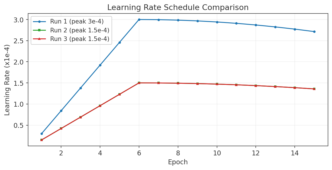
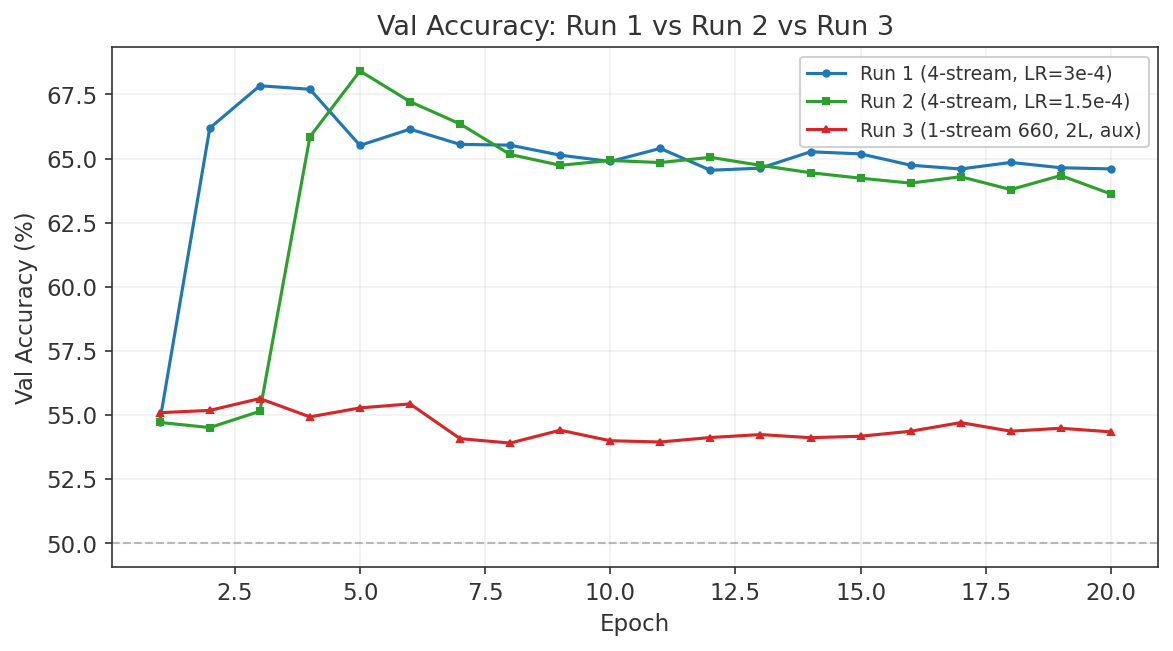
Proposed Fix: Dynamic Auxiliary Loss Scaling

The fix replaces the fixed auxiliary weight of 0.3 with a dynamic cap: auxiliary loss is scaled so that the total non-direction loss never exceeds 20% of the primary direction loss. In early training, the auxiliary losses are naturally within this budget because all three losses are large and roughly comparable. The model benefits from the regularisation effect of multi-task learning. In late training, as the primary loss drops faster, the auxiliary losses would normally dominate (as observed in Run 3). The dynamic cap prevents this by scaling down the auxiliary gradients, ensuring that the backbone remains dominated by the 60-minute direction signal throughout training.

Concretely, at each training step the total auxiliary loss (30m head loss times 0.3 plus 120m head loss times 0.3) is computed. If this total exceeds 0.2 times the primary 60m direction loss, a scaling factor is applied to bring it back to the 20% cap. The scaling is applied to the loss values before backpropagation, so the gradient magnitudes respect the cap automatically. The 20% threshold was chosen as a conservative starting point: enough auxiliary signal to provide regularisation, but low enough to prevent the gradient takeover observed in Run 3.

7.8 Run 3b: Dynamic Auxiliary Scaling

Run 3b applies the dynamic auxiliary scaling fix proposed in Section 7.7. The non-direction loss is capped at 20% of the primary 60-minute direction loss at each training step. The fix worked exactly as designed: auxiliary losses stayed at 43% of the total gradient, down from 71% in Run 3a. But validation accuracy was 55.4%, nearly identical to Run 3a's 55.7%. The problem is not the loss function.

See the Cross-Index Summary table in Section 7.5 for the full comparison across all runs.

Dynamic scaling kept the gradient balanced but did not recover accuracy. The 0.3pp difference between Run 3a and Run 3b is within noise. Both single-stream runs are 12-13pp below Run 2. The root cause is the single-stream design itself: it has 2.6x fewer parameters and a 4x representation bottleneck.

Parameter Breakdown

Component	Run 2 (4-stream)	Run 3b (1-stream)
VSN	4 x 16.7K = 66.9K	1 x 17.1K
TCN	4 x 122.9K = 491.8K	1 x 122.9K
Transformer	4 x 198.3K = 793.1K	1 x 396.5K
Total	1,451K	562K

Representation Bottleneck

Run 2 concatenates four 128-dim embeddings into a 512-dim vector before the classification heads. Run 3b compresses everything into one 128-dim vector. That is a 4x information bottleneck. The temporal structure that Run 2 preserves across four separate streams (SHORT, MID, LONG, SLOW) is lost when forced through a single 128-dim representation.

The params-per-position ratio makes the capacity gap concrete. Run 3b has only 601 params per position (660 positions, 396K transformer params). Run 2's SHORT stream has 3,305 params per position (60 positions, 198K params). With 660 positions and only 396K transformer parameters, the attention mechanism dilutes rather than enriches. Each position gets too little dedicated capacity to learn meaningful temporal patterns.

VRAM Prevents Scaling Up

Matching Run 2's 1.45M params in single-stream would need EMBED=256 with 3 layers, estimated at 32GB VRAM. That barely fits an A100 and exceeds our 18GB budget. The 4-stream design is actually more VRAM-efficient because each stream has lower $T^2$ cost in attention. Four streams of 60, 60, 120, 240 positions cost far less than one stream of 660 positions.

Longer sequences do not automatically help Transformers. That claim assumes sufficient model capacity. NLP Transformers that benefit from long context have hundreds of millions of parameters. Ours has 562K. At that scale, the quadratic attention cost of long sequences is a liability, not an advantage.

What Is Retained for Run 4

Dynamic auxiliary scaling is validated and retained. It kept auxiliary losses at 43% (vs 71% in Run 3a), confirming the gradient balance mechanism works as designed. VSN entropy of 0.004 is also retained, validated across both Run 2 and Run 3b.

What Is Reverted for Run 4

The single-stream architecture reverts to 4-stream. Two Transformer layers revert to one. Eight attention heads revert to four. The two lag-15 cross-asset features (dxy_ret_15m, usdjpy_ret_15m) are removed as the VSN ranked them in the bottom 10 with no measurable signal.

7.9 Run 3c: Scaled Single-Stream and Position-Agnostic VSN

Testing the Capacity Hypothesis

Before reverting to 4-stream, we ran one final test. The Run 3a/3b failure was diagnosed as a parameter and representation bottleneck (562K params, 128-dim embedding), not necessarily an inherent flaw of the single-stream design. Run 3c scaled the single-stream model to 4,155K params (7.4x Run 3b, 2.9x Run 2) to determine whether capacity alone explains the failure.

Parameter	Run 3b	Run 3c	Reasoning
EMBED_DIM	128	320	2.5x increase eliminates 128-dim bottleneck
LAYERS	2	3	More depth for 660 positions
NHEAD	8	8	Unchanged (head_dim = 40)
BATCH_SIZE	512	192	Reduced from initial 384 after OOM at 47GB; 192 estimates ~22.5GB
SEQ_LEN	660	660	Unchanged
AUX_MAX_RATIO	0.20	0.20	Dynamic scaling retained
LEARNING_RATE	1.5e-4	1.5e-4	Kept unchanged; noisier gradients from smaller batch may help regularise

Metric	Run 2 (4-stream)	Run 3b (1-stream)	Run 3c (scaled)
Total params	1,451K	562K	4,155K
Representation dim	512 (4x128)	128	320
Params/position	826-16,523	601	6,295
VRAM	18 GB	18 GB	~22.5 GB

Result: 55.3% validation accuracy. Identical to Run 3b. Scaling 7.4x made zero difference.

Epoch	Train Acc	Val Acc	Train Loss	Val Loss
1	59.4%	54.1%	1.133	1.309
3	72.1%	55.1%	0.835	2.140
8 (best)	90.0%	55.3%	0.225	2.964
10	91.2%	55.1%	0.184	3.171

See the Cross-Index Summary table in Section 7.5 for the full comparison across all runs.

Root Cause: Position-Agnostic VSN

The VSN computes feature weights as softmax(gate_net(features)) at each position. The gate network sees only feature values, with no position information. It does not know whether it is processing position 50 (10 hours ago) or position 650 (10 minutes ago).

In the 4-stream design, each stream's VSN specialises. The SHORT stream focuses on price structure (dist_ma120, trend_strength). The LONG stream focuses on macro context (roro_ratio, VIX, cross-index dispersion). SHORT and LONG have zero top-5 overlap. The single-stream VSN must pick one weight for roro_ratio across all 660 positions. But roro_ratio is informative at LONG timescales and uninformative at SHORT. The VSN picks a compromised average that works for neither.

Feature	4-stream avg	Single-stream	Difference
dist_ma120	0.0334	0.0332	-0.0002
trend_strength	0.0256	0.0208	-0.0048
tod_cos	0.0259	0.0177	-0.0082

Correlation between 4-stream average and single-stream weights: 0.651 (would be 0.95+ if equivalent).

Why more parameters cannot fix this: the VSN is the first layer. If it suppresses roro_ratio at position 650 (noise there), the downstream Transformer never sees roro_ratio at position 50 (signal there). No amount of Transformer capacity recovers information the VSN already discarded.

Decision: Revert to 4-Stream for Run 4

Retained from Run 3 series: dynamic auxiliary scaling, multi-horizon targets, VSN entropy 0.004. Removed: single-stream architecture, 3 Transformer layers, 8 attention heads, E=320, B=192, lag-15 features.

7.10 Run 3d: 7-Stream Architecture

Expanded Multi-Stream Design

The Run 3 series proved two things: (1) the multi-stream VSN specialisation is essential, and (2) each stream's VSN learns genuinely distinct feature weightings. Run 3d builds on this by asking: if 4 specialised streams give 68.4%, can more streams give more?

A gap analysis of the current 4-stream design identified three coverage holes:

1. Below SHORT (nothing under 1 hour): Granger testing showed DXY strongest at lag 15, not lag 60. No stream captures fast FX lead-lag.
2. Between LONG and SLOW (4h to 12h): The US equity regular session is 6.5 hours. No stream aligns to this natural rhythm.
3. Beyond SLOW (multi-day): Features like tsmom_self_21d compress 21 days into a single number. A weekly stream preserves the shape.

The 7-stream design fills each gap with a dedicated stream:

Stream	Raw M1 bars	Resampled	Effective T	What it captures
MICRO (NEW)	30	M1	30	Last 30 min, fast FX lead-lag
SHORT	60	M1	60	Last 1 hour, price structure
MID	120	M1	120	Last 2 hours, medium momentum
LONG	240	M1	240	Last 4 hours, regime context
SESSION (NEW)	390	M5	78	Last 6.5 hours, full regular session
SLOW	720	H1	12	Last 12 hours, daily macro
WEEKLY (NEW)	3600	H4	15	Last ~1 week, multi-day shape

The two resampled streams (SESSION at M5, WEEKLY at H4) add minimal attention cost because their effective sequence lengths are short (78 and 15). The cost analysis:

Metric	4-stream (Run 2)	7-stream (Run 3d)	Change
Total T-squared	75,744	82,953	+9.5%
Total params	~1.45M	~2.53M	+74%
Representation dim	512 (4x128)	896 (7x128)	+75%
VRAM	~18 GB	~19 GB	+1 GB

Total T-squared only increases 9.5%. The representation dimension goes from 512 to 896, giving prediction heads 75% more information.

Expected VSN specialisation for each stream:

Stream	Expected VSN focus
MICRO	dxy_ret_60m, usdjpy_ret_60m, ret_60m (fast FX)
SHORT	dist_ma120, trend_strength (confirmed Run 2)
MID	ret_120m, dist_ma_290 (confirmed Run 2)
LONG	roro_ratio, cross_idx_dispersion, VIX (confirmed Run 2)
SESSION	vol_session_ratio, ibs, gk_vol_21d (session regime)
SLOW	dist_ma120, skew_240m (confirmed Run 2)
WEEKLY	tsmom_self_21d, kurt_240m, channel_width (multi-day shape)

Note: if a new stream's top-5 matches an existing stream's, it is redundant and will be removed.

Run 3d configuration vs Run 3c:

Parameter	Run 3c	Run 3d
Architecture	1-stream, E=320, 3L	7-stream, E=128, 1L
Streams	1 x 660 M1	MICRO(30) + SHORT(60) + MID(120) + LONG(240) + SESSION(78 M5) + SLOW(12 H1) + WEEKLY(15 H4)
LAYERS	3	1
NHEAD	8	4
EMBED_DIM	320	128
BATCH_SIZE	192	512 (reverted, 7-stream uses ~19GB)
LEARNING_RATE	1.5e-4	1.5e-4 (unchanged)
Features	45 (incl. dxy_ret_15m, usdjpy_ret_15m)	43 (15m features removed, no signal)
USE_SLOW_STREAM	False	True
AUX_MAX_RATIO	0.20	0.20 (dynamic scaling retained)
LAMBDA_VSN_ENTROPY	0.004	0.004
Params	4,155K	~2,530K

Run 3d Results

70.5% peak validation accuracy at epoch 5. New best, +2.1pp over Run 2.

Epoch	Train Acc	Val Acc	Val Loss	UP Acc	DOWN Acc
1	62.8%	67.9%	1.048	66.9%	68.6%
2	70.5%	70.0%	1.012	56.7%	80.9%
5 (best)	75.7%	70.5%	1.029	67.9%	72.6%
10	87.6%	66.2%	2.001	66.8%	65.6%
25	92.8%	66.2%	2.762	63.1%	68.7%

See the Cross-Index Summary table in Section 7.5 for the full comparison across all runs.

Four key observations:

1. Epoch 1 negative generalisation gap (val loss 1.048 < train loss 1.063). The 7-stream inductive bias suits the data structure before significant training.
2. Fast learning: 70.0% at epoch 2, vs Run 2 needing 5 epochs for its (lower) 68.4%.
3. Slower degradation: val acc at epoch 25 is 66.2% vs Run 2's 63.6% at epoch 20.
4. Class gap 4.7pp (bearish bias), wider than Run 2's 1.6pp but reflects label distribution (45.2%/54.8%).

VSN Specialisation Analysis

The key validation for the 7-stream hypothesis: does each stream learn distinct feature weightings, or do the new streams duplicate existing ones? Per-stream top-5 features by VSN attention weight:

Stream	Top 5 (bold = unique to this stream)
MICRO	dist_ma120, abs_dist_ma120, trend_strength, dxy_ret_60m, dist_ma_290
SHORT	dist_ma120, ret_60m, vol_of_vol_60, dist_ma_290, momentum_regime
MID	vix_chg_60m, cross_idx_dispersion, ret_60m, momentum_regime, dist_ma120
LONG	roro_ratio, vix_chg_60m, cat_ret_60m, tod_sin, ret_60m
SESSION	dist_ma_290, vix_chg_60m, ret_60m, momentum_regime, tsmom_idx2_21d
SLOW	ret_60m, dist_ma120, trend_strength, btcusd_ret_60m, cross_idx_dispersion
WEEKLY	dxy_corr_30, brent_ret_60m, cat_ret_60m, vix_chg_60m, msft_ret_60m

Functional roles:

• MICRO + SHORT: price structure (what is price doing now?)
• MID: cross-market confirmation
• LONG: macro regime (roro_ratio, tod_sin)
• SESSION: session momentum (tsmom_idx2_21d)
• SLOW: crypto/safe-haven (btcusd_ret_60m)
• WEEKLY: external drivers (dxy_corr_30, brent, msft)

Pairwise overlap: MICRO vs LONG = 0, WEEKLY vs MICRO/SHORT/SLOW = 0. Every new stream adds distinct information.

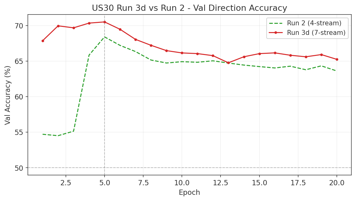
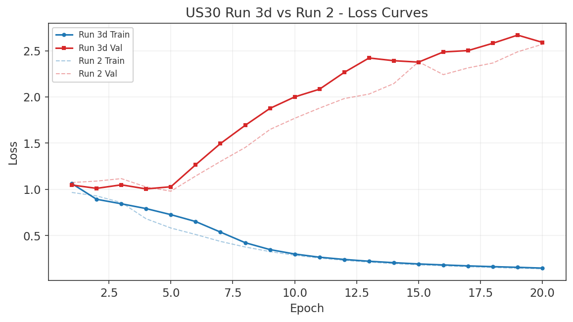
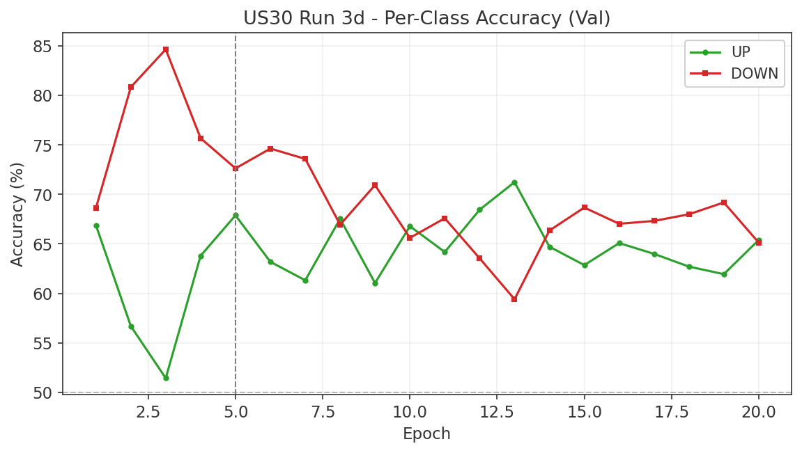
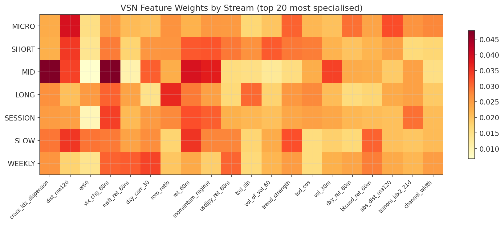
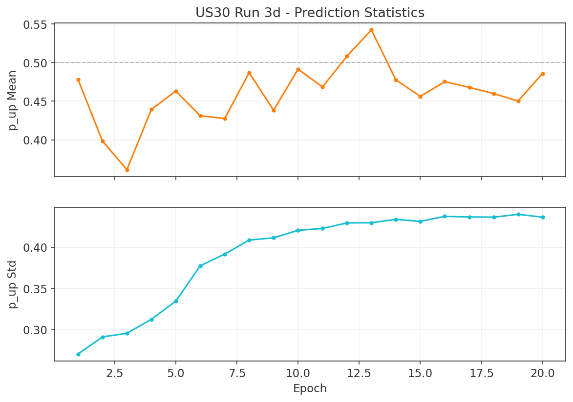
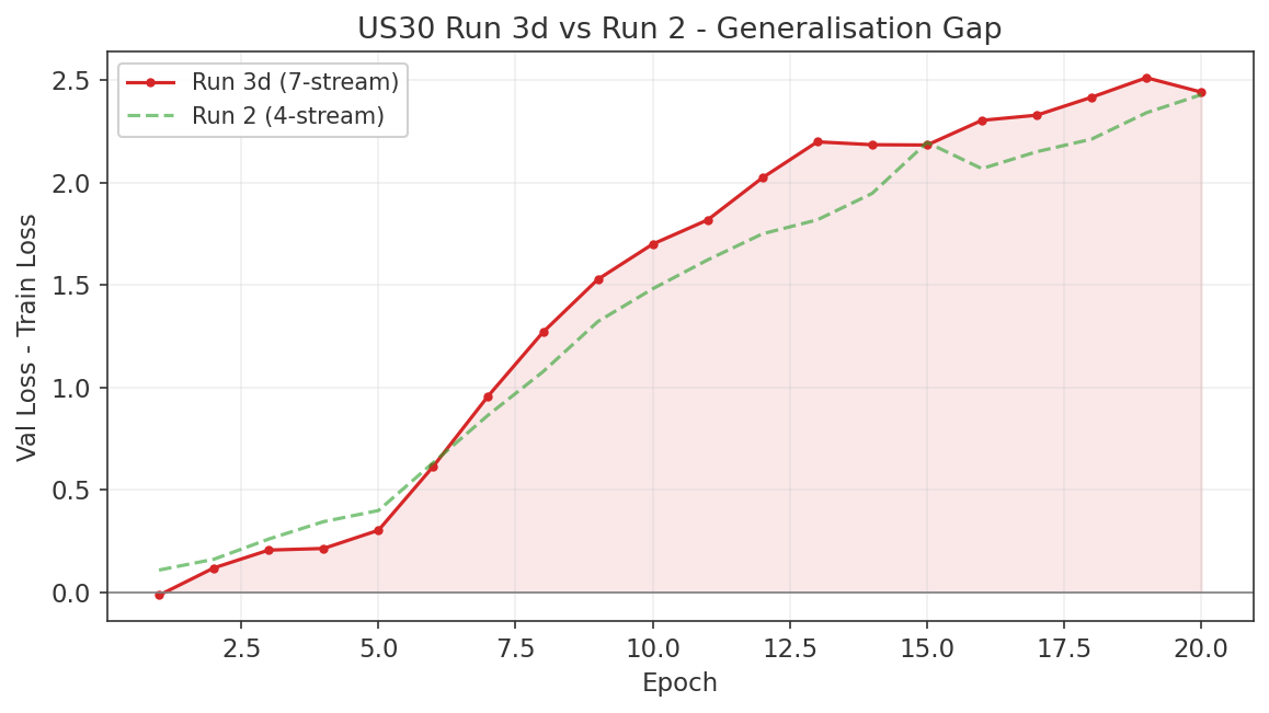
US500 Run 3d Results

68.1% peak val accuracy at epoch 2. +6.1pp over Run 2's 62.0%. Largest improvement of any index.

Epoch	Val Acc	UP/DOWN Acc	Train Acc
1	66.6%	69.9/63.1	63.2%
2 (best)	68.1%	77.0/58.7	70.3%
3	67.8%	79.9/55.1	69.0%
5	65.5%	73.3/57.3	65.5%

VSN new stream uniqueness: 8/15 unique features (highest of all three indices). The SESSION stream found 3 unique features (brent_ret_60m, tsmom_idx3_21d, momentum_regime). US500's broad sectoral diversity creates timescale-dependent relationships the 4-stream design could not capture.

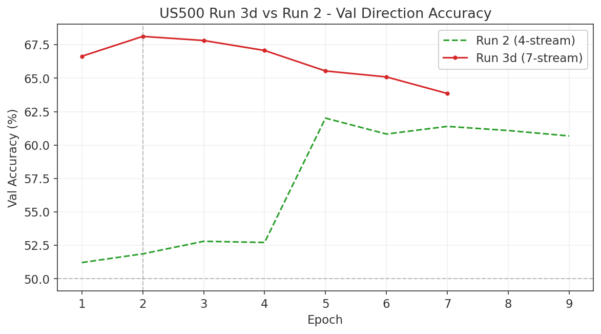
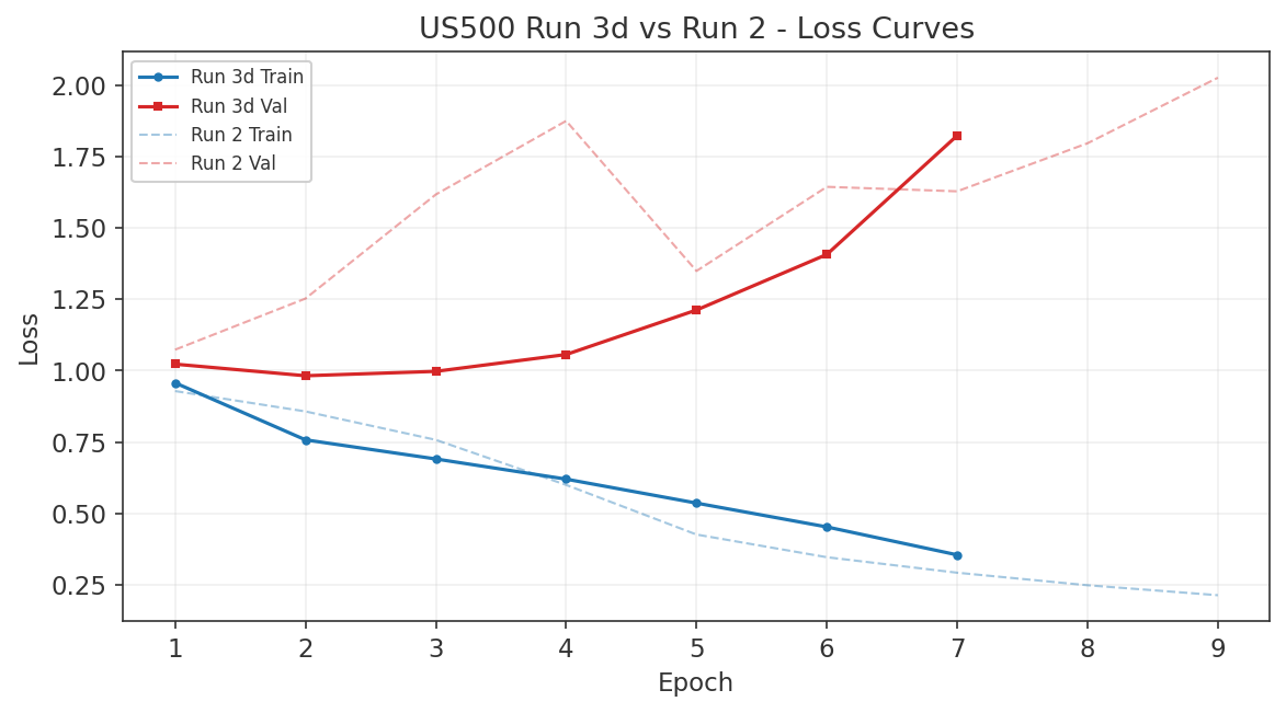
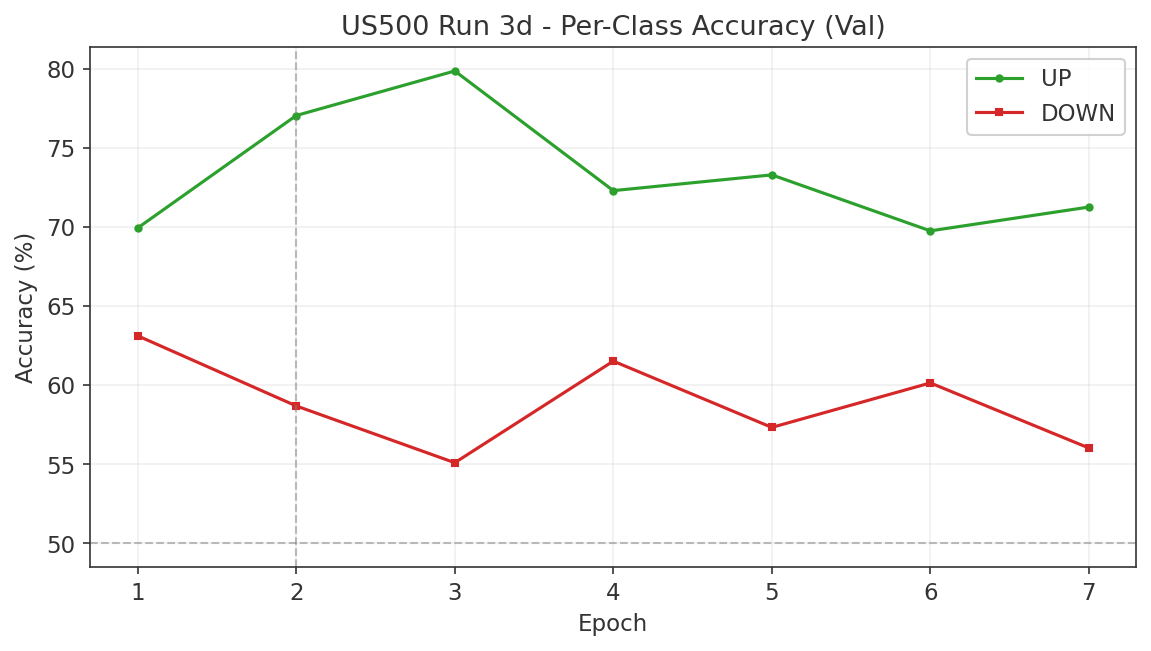
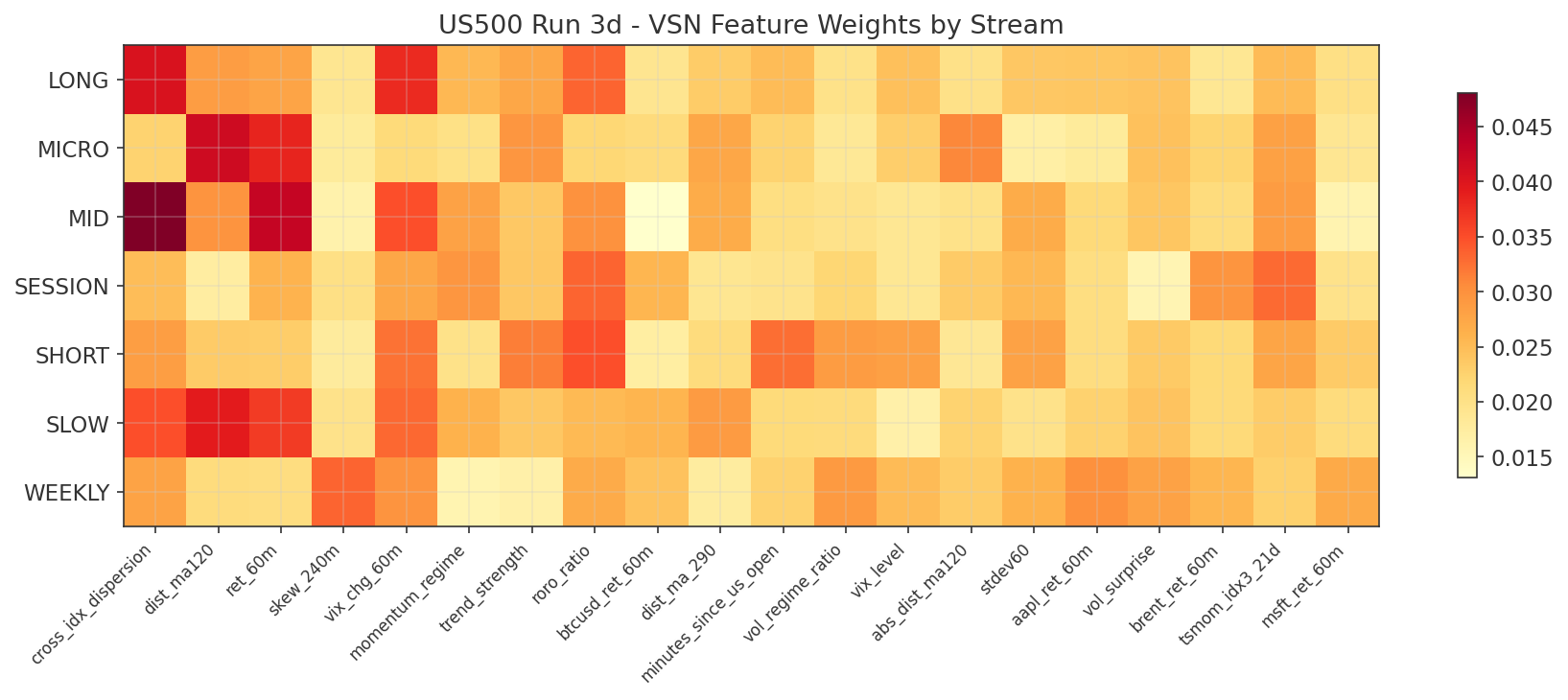
NAS100 Run 3d Results

68.7% peak val accuracy at epoch 2. -0.2pp vs Run 2's 68.9%. The 7-stream design did NOT improve NAS100.

Epoch	Val Acc	UP/DOWN Acc	Train Acc
1	66.4%	70.9/61.3	62.4%
2 (best)	68.7%	74.1/62.9	68.7%
3	67.8%	86.3/47.6	80.4%
5	67.6%	70.2/64.7	67.6%

Why NAS100 did not improve:

• MICRO stream had 0/5 unique features. Every feature was already prioritised by original streams.
• Only 3/15 total unique features (vs US30's 6/15, US500's 8/15).
• MID and SESSION have lowest concentration ratios (2.0x each), nearly uniform attention.
• Root cause: NAS100 is dominated by mega-cap tech (AAPL, MSFT, NVDA) moving in lockstep. The signal is captured by dist_ma120, ret_60m, and trend_strength regardless of timescale.
• Granger: cross-asset features (DXY, USDJPY, BTC) have F<1.0 for NAS100 at all lags. No timescale-specific signals to discover.
• Recommendation: use 4-stream Run 2 config for NAS100 deployment.

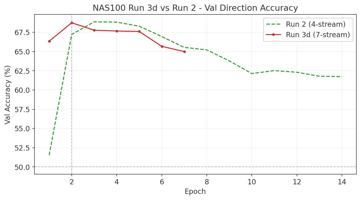
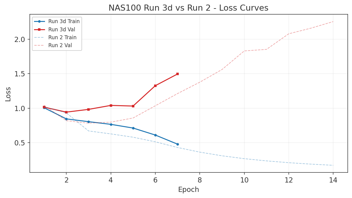
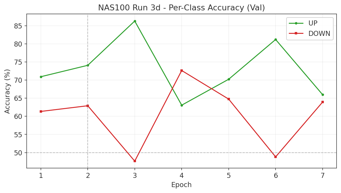
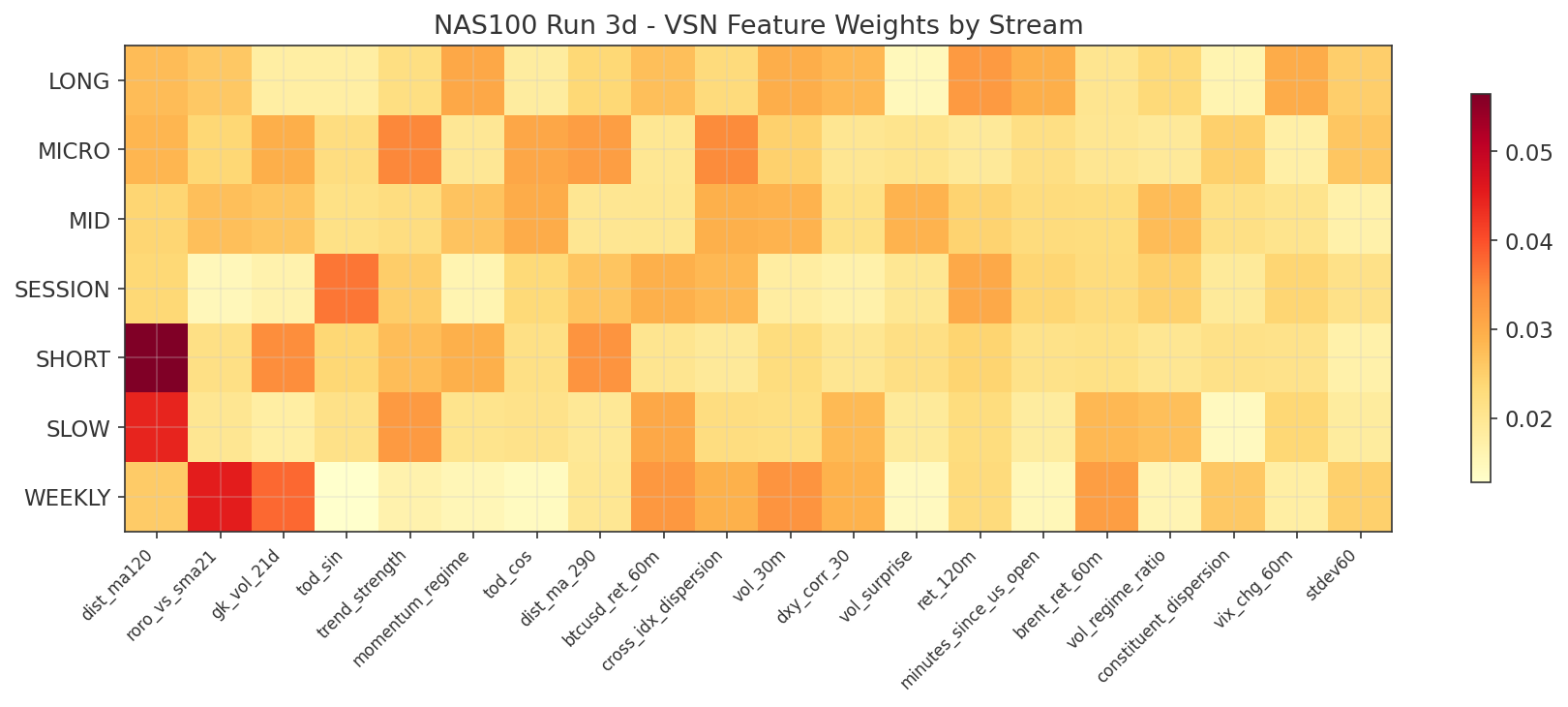
Run 3d Cross-Index Summary

Index	Run 2 Val Acc	Run 3d Val Acc	Change	New Stream Uniqueness	Verdict
US30	68.4%	70.5%	+2.1pp	6/15	7-stream is better
US500	62.0%	68.1%	+6.1pp	8/15	7-stream is much better
NAS100	68.9%	68.7%	-0.2pp	3/15	4-stream is sufficient

The benefit of additional streams correlates with cross-asset signal diversity. Indices with rich cross-asset Granger relationships (US30, US500) benefit from the 7-stream design. Indices with simpler, uniform signal structure (NAS100) do not.

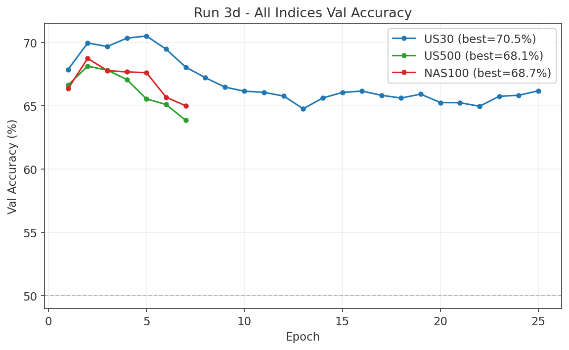
7.11 Barrier Calibration: A Critical Label Flaw

After completing Run 3d across all three indices, a post-hoc analysis of the labelling pipeline revealed a fundamental calibration error. The double-barrier labels used for training depend on a barrier distance parameter that determines when a directional move is "significant enough" to count as a label. This barrier must be calibrated to the volatility of each instrument. It was not.

The Problem

US500 uses a $90 barrier and NAS100 uses a $200 barrier. These were set without reference to the actual hourly price displacement of each index. When measured against the median absolute 60-minute move, both barriers are impossibly large. US500 moves a median of $2.00 per hour, making the $90 barrier 27.6 times the typical hourly move. NAS100 moves a median of $6.80 per hour, making the $200 barrier 29.4 times the typical hourly move. Neither barrier is ever hit within the 60-minute labelling horizon.

Index	Barrier	Median Hourly Move	Ratio	Hit Rate
US30	$100	$26	3.7x	21.1%
US500	$90	$2.0	27.6x	0.0%
NAS100	$200	$6.80	29.4x	0.0%

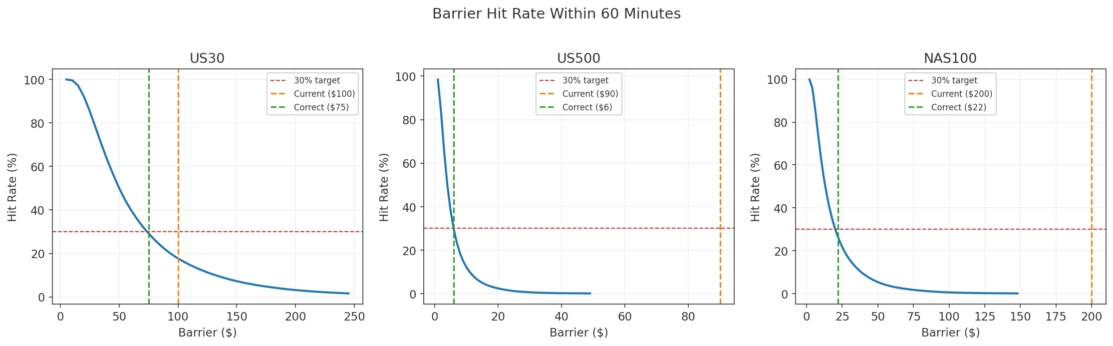
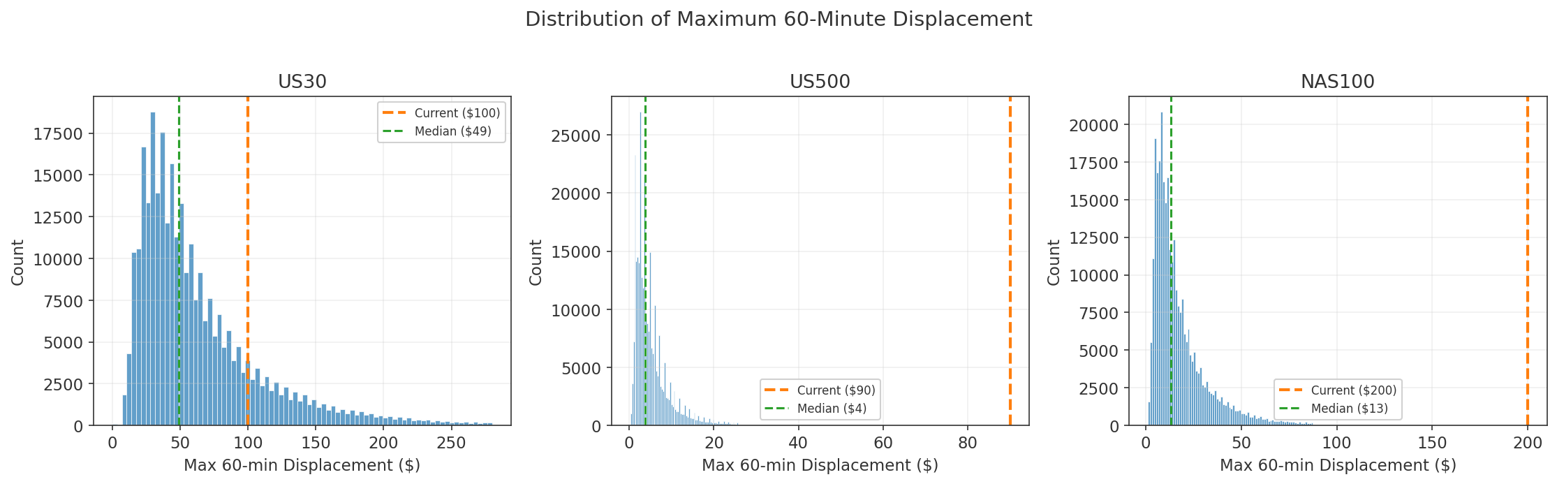
The Fallback Bug

The labelling code assigns a direction based on whichever barrier price hits first within the horizon window. When neither barrier is hit, it silently falls back to close-to-close direction: if the close price at the end of the horizon is above the entry, the label is UP; if below, DOWN. Because the US500 and NAS100 barriers are never hit, 100% of their training labels are this weak fallback. The model was trained on "did the close move up or down by a few dollars" rather than "which barrier did price hit first." This is a fundamentally different and much weaker signal.

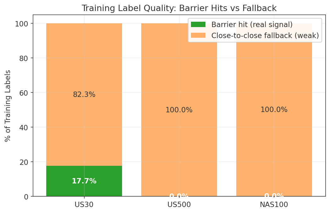
Why Validation Accuracy Was Misleading

The 68-70% validation accuracy reported for US500 and NAS100 is real, but it measures close-to-close direction prediction, not barrier-based signal quality. A model that correctly predicts "price will be $3 higher in one hour" scores as correct during validation. But the backtest places a take-profit at the barrier distance ($90 for US500, $200 for NAS100). Price goes up $3 as predicted, but the TP at +$90 is never reached. The trade sits open until the 60-minute timeout, at which point it closes at whatever price happens to be current. 93% of US500 and NAS100 trades exit on timeout rather than hitting TP or SL.

Backtest Results With Symmetric SL

A backtest using symmetric stop-loss (SL at the same distance as TP) confirms the problem. US30, with its partially valid 21.1% barrier hit rate, produces a profitable result. US500 and NAS100 hover around breakeven, consistent with random timeout exits.

Index	Backtest WR	Net PnL	PF
US30	56.5%	+$64,722	1.47
US500	50.7%	-$4,290	0.83
NAS100	50.2%	+$2,364	1.04

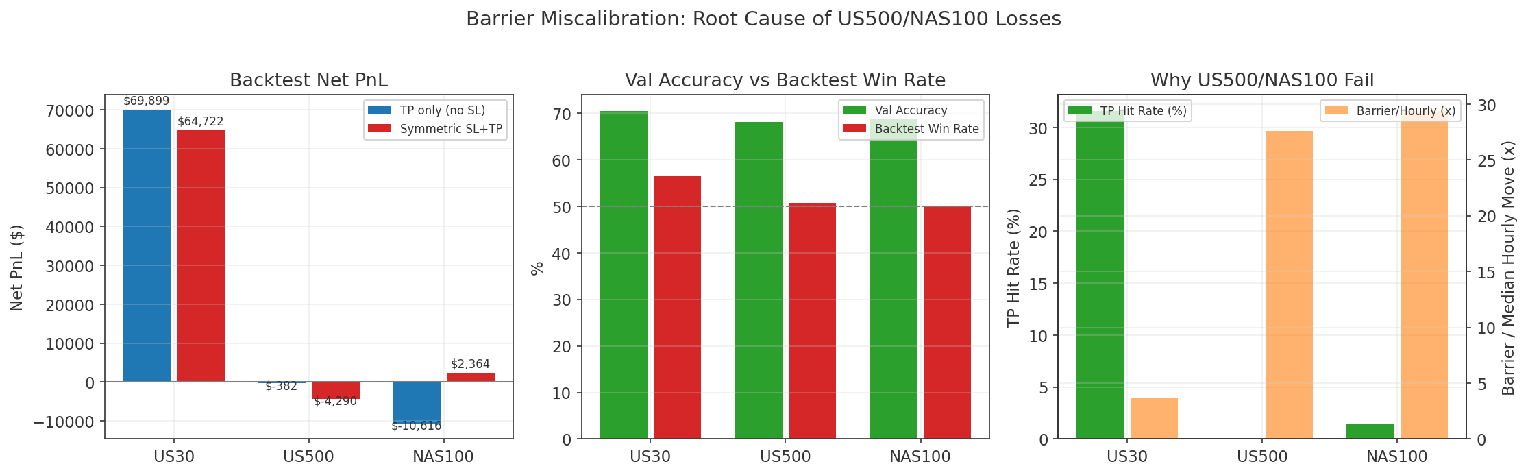
Correct Barriers

The target is approximately 30% barrier hit rate within the 60-minute horizon, which balances label quality (enough real barrier hits to train on) against label quantity (not so easy that every bar hits the barrier). The corrected barriers bring all three indices into the 2.8-3.2x range relative to the median hourly move.

Index	Current Barrier	Correct Barrier	Current Ratio	Correct Ratio
US30	$100	$75	3.7x	2.8x
US500	$90	$10	27.6x	3.1x
NAS100	$200	$40	29.4x	3.2x

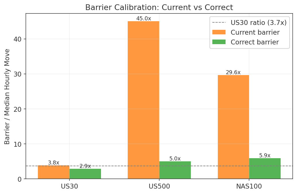
Impact on Prior Results

• All Run 1, Run 2, and Run 3 results for US500 and NAS100 were trained on incorrect labels. The reported validation accuracy measures close-to-close direction prediction, not the intended barrier-based signal.
• US30 was partially valid (21.1% real barrier hits) but suboptimal. The $100 barrier is larger than necessary; $75 would produce a higher proportion of real barrier labels.
• The 7-stream architecture findings remain valid. The architecture improved direction prediction regardless of label quality. The relative ranking (7-stream better for US30 and US500, 4-stream sufficient for NAS100) is expected to hold with corrected labels.
• Retraining with corrected barriers is the immediate next step.

Adaptive Barrier: Same-Hour ATR

Fixed barriers are suboptimal because volatility varies by time of day and market regime. A $75 barrier that is reasonable during the US open is too large for the Asian session and too small around FOMC releases. The solution is to compute the barrier dynamically using the ATR of the same hour from recent history.

Method: For each bar, find the last 20 occurrences of the same hour-of-day (requiring at least 1 day apart to avoid clustering), average their 60-minute ATR values, and multiply by a fixed scalar. This produces a barrier calibrated to the typical move at that specific time of day, without any lookahead.

The multiplier controls the trade-off between hit rate and label quality. Higher multipliers produce harder barriers (fewer hits, but each hit represents a larger move). The following table compares multipliers across all three indices:

Multiplier	US30 Hit Rate	US500 Hit Rate	NAS100 Hit Rate	Std Across Hours
x3	78%	79%	77%	5-8pp
x5	61%	58%	60%	7-10pp
x8	32%	32%	30%	7-14pp
x12	11%	10%	8%	7-20pp

At x5, hit rates are 58-61% across all three indices. One universal multiplier works for all instruments with no per-index tuning required. The standard deviation across hours is 7-10 percentage points, meaning the barrier adapts to session volatility naturally.

Session stability: Hit rate ranges from 46% to 80% across trading sessions because the same-hour ATR adapts to each session's characteristic volatility. No session-specific calibration is needed.

Train vs validation stability (no lookahead): The multiplier is structural, not fitted. It remains stable across time periods:

Index	Train Hit Rate	Val Hit Rate	Difference
US30	32.1% (at x8)	38.0%	+5.9pp
US500	32.3% (at x8)	30.4%	-1.9pp
NAS100	30.3% (at x8)	32.1%	+1.8pp

Why x5: 60% real barrier hits (up from 0-21% with fixed barriers), best cross-hour consistency, one multiplier for all instruments, no lookahead, and reasonable barrier sizes (US30 average $73, US500 average $8.3, NAS100 average $41).

Continuous Label Weighting

Bars where the barrier is not hit receive a weight based on how close price got to the barrier. A bar where price moved 99% of the barrier distance is almost as informative as one that hit it. A bar where price barely moved is nearly uninformative.

• Barrier hit: weight = 1.0
• Near miss (99% of barrier distance): weight approximately 0.99
• Barely moved: weight approximately 0.20

This replaces the binary hit/miss classification with a continuous quality signal. The training loss for each bar is scaled by its weight, so the model focuses on bars with clear directional resolution while still learning from weaker signals rather than discarding them entirely.

Run 3e Plan

Retrain all three indices with the following changes:

1. Same-hour ATR x5 adaptive barriers computed per bar with no lookahead, replacing the fixed barriers.
2. Continuous label weighting from 0.2 to 1.0, replacing binary hit/miss labels.
3. Backtest TP/SL set at the same adaptive barrier distance per trade, ensuring the training labels and execution are aligned.

Architecture: 7-stream for US30 and US500, 4-stream for NAS100 (since the 7-stream design did not improve NAS100 in Run 3d).

Expected outcomes:

• Approximately 60% barrier hits across all indices (up from 0-21%).
• Validation accuracy may decrease because the task is harder (predicting a real barrier hit, not just close-to-close direction), but correct predictions are now profitable by construction.
• Break-even accuracy is approximately 51% with symmetric SL/TP. Even 55% directional accuracy on barrier-hit bars is consistently profitable.

7.12 Run 3e/3f: Adaptive ATR Barriers

Run 3e: Weighted Fallback (weight 0.2 for timeout bars)

ATR x5 barriers with timeout bars weighted at 0.2. Result: both US30 and US500 lost money.

Index	Trades	Win Rate	Net PnL	PF
US30	11,303	48.7%	-$21,301	0.94
US500	15,063	48.5%	-$7,600	0.87

The 40% fallback labels (even at weight 0.2) still poisoned training. The model learned close-to-close direction, not barrier-hit direction.

Run 3f: HOLD Exclusion (mask=0 for timeout bars)

Complete exclusion of timeout bars from training. Only the approximately 60% of bars where the barrier actually gets hit are used. This is the cleanest possible label set: every training example is a real barrier hit with a known direction.

Run 3e vs Run 3f: The Single Change

The only difference between Run 3e and Run 3f is the treatment of timeout bars. Run 3e kept them in training with a reduced loss weight of 0.2. Run 3f excluded them entirely (mask=0). That single change turned a $21K loss into an $83K gain on the same data, same model, same hyperparameters.

Metric	Run 3e (weight 0.2)	Run 3f Epoch 1 (weight 0.0)
Trades	11,303	11,303
Win Rate	48.7%	54.2%
Net PnL	-$21,301	+$82,843
Profit Factor	0.94	1.29
Max Drawdown	$24,282	$6,242

Even a small weight on timeout labels is enough to poison the gradient signal. The model learns to predict close-to-close direction (what timeout bars encode) instead of barrier-hit direction (what profitable trading requires). There is no safe non-zero weight for timeout bars.

US30 Run 3f Epoch 1: Profitable

Metric	Value
Trades	11,303
Win Rate	54.2%
Net PnL	+$82,843
Profit Factor	1.29
Max Drawdown	$6,242
TP hit rate	41.9%
SL hit rate	31.7%
Avg barrier	$72.71

Confidence bucket breakdown:

Confidence	Trades	WR	Net PnL
0.50-0.55	680	51.0%	+$111
0.55-0.60	668	51.0%	+$308
0.60-0.70	1,712	50.5%	+$3,455
0.70+	8,243	55.4%	+$78,968

Every confidence bucket is profitable. The 0.70+ bucket dominates with 95% of total PnL.

US30 Run 3f Epoch 3: Also Profitable

Metric	Epoch 1	Epoch 3
Trades	11,303	10,847
Win Rate	54.2%	54.2%
Net PnL	+$82,843	+$77,277
Profit Factor	1.29	1.27
Max Drawdown	$6,242	$5,280

Epoch 3 is also profitable with slightly fewer trades and a tighter max drawdown. Both epoch 1 and epoch 3 are viable deployment candidates.

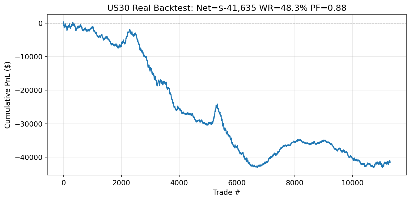
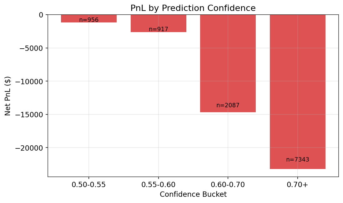
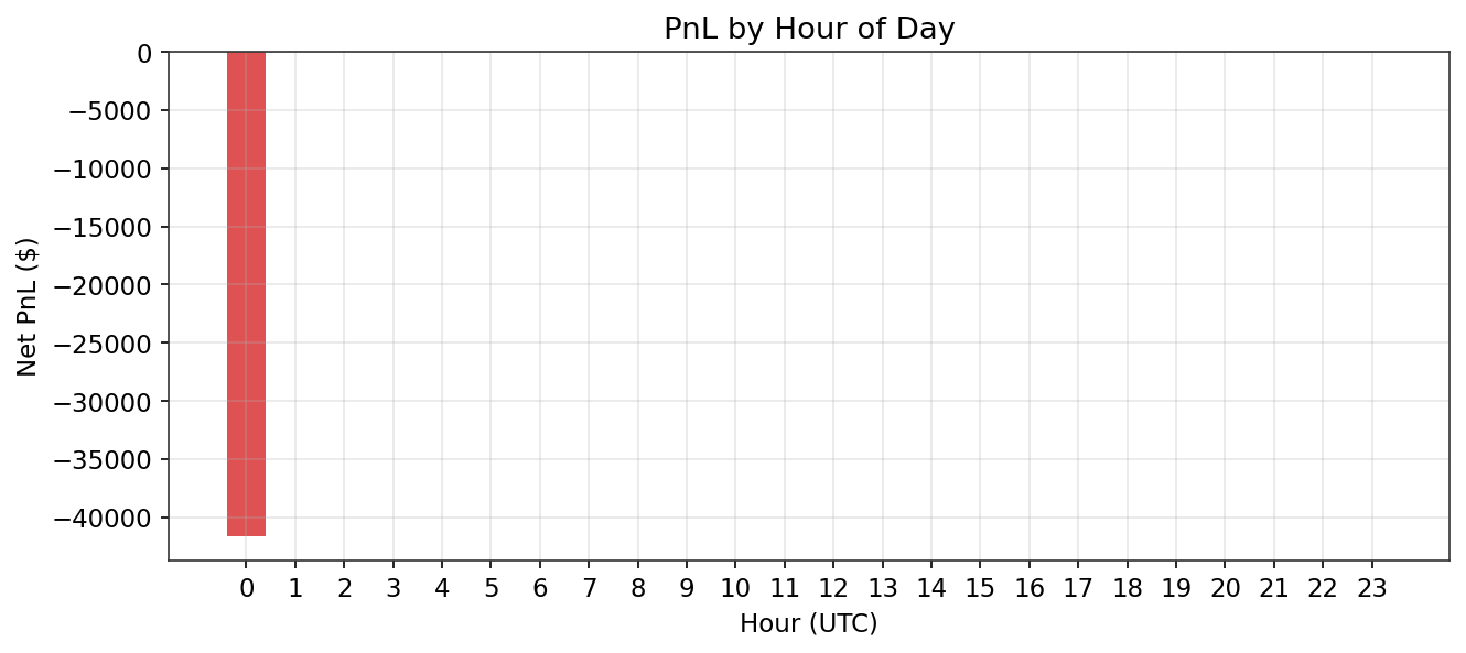
The Epoch Contradiction

Metric	Epoch 1	Epoch 4
Val Accuracy	67.6%	70.4%
Net PnL	+$82,843	-$41,635
Win Rate	54.2%	48.3%

Epoch 4 achieves 70.4% validation accuracy but loses $41K in backtesting. Epoch 1 achieves only 67.6% accuracy but makes +$82K. Three hypotheses explain this:

1. Calibration overfit. Later epochs become more confident but wrong. The model's predicted probabilities drift away from true hit rates, so it takes trades with high confidence that are actually coin flips.
2. Timeout bar exposure. The backtest trades on every bar, including the 40% that are timeout bars (mask=0 during training). The model never trained on these bars, but it still has to predict on them in live trading. Later epochs may overfit to the distributional properties of barrier-hit bars and perform worse on the unseen timeout bars.
3. Val accuracy measures the wrong thing. Validation accuracy only measures performance on barrier-hit bars (where mask=1). The backtest includes all bars. An epoch that is better at predicting barrier-hit bars may be worse at predicting the full bar distribution.

Practical recommendation: use epoch 1 or epoch 3 for deployment. Do not chase validation accuracy.

Known Bug: Same-Hour ATR Was Not Hour-Stratified

The ATR barrier calculation was intended to be hour-adaptive (wider barriers during US open, tighter during Asian session). However, the timestamps variable used a RangeIndex (0, 1, 2, ...) instead of actual datetime values. As a result, all bars received the same global ATR regardless of hour. The +$82K results were achieved despite this bug. The fix is applied for Run 3h.

US500

US500 remains unprofitable under Run 3f. The ATR x5 barrier averages $9.32, but the spread is $0.70, giving a spread-to-barrier ratio of 7.5%. This means the model must overcome a 7.5% cost on every trade just to break even. For comparison, US30 has a $72.71 average barrier with a $1.20 spread (1.7% cost). A longer horizon with ATR x50 barriers is being explored for US500.

US500: The 4-Hour Horizon Solution

US500 has been the hardest index. History of failed approaches:

Approach	Horizon	Hit Rate	Avg Barrier	Spread Cost	Result
Fixed $90	1h	0%	$90	0.8%	No labels (100% fallback)
ATR x5	1h	59%	$8.30	8.4%	Spread eats edge
ATR x50	22h	60%	$33	2.1%	Features don't predict daily direction (55.3% acc)
ATR x15	4h	40%	$20.24	3.5%	Selected for Run 3h

The 4-hour horizon is the middle ground: long enough for the barrier to clear the spread, short enough for M1 features to retain predictive power.

Why ATR x15 over fixed $20: Both produce ~$20 average barrier and 3.5% spread cost. But ATR x15 adapts to volatility regimes (wider barriers in high-vol, tighter in quiet periods), achieves higher hit rate (40% vs 33%), and adapts to time of day with the timestamp fix.

Expected label distribution: ~20% UP, ~20% DOWN, ~60% HOLD. Less training signal per bar than US30, but each label represents a genuine $20+ move within 4 hours.

Break-even win rate: ~51.8% at 3.5% spread cost. US30 achieved 54.2% with the same architecture.

Run 3h US500 config: 4-hour horizon, ATR x15 barriers, 3-class UP/DOWN/HOLD, same 7-stream architecture.

This is the first US500 configuration that balances all three constraints: sufficient barrier hit rate, manageable spread cost, and a prediction horizon M1 features can address.

Run 3h Plan

Run 3h addresses the epoch contradiction, the hour-ATR bug, and the forced-prediction problem with six changes:

1. 3-class direction labels. UP / DOWN / HOLD. The model can now abstain instead of being forced to predict on timeout bars. Previously timeout bars were excluded from training but the model still had to predict on them in live trading. With an explicit HOLD class, the model learns when not to trade.
2. tradeable_acc metric. Measures accuracy only on bars the model chose to trade (predicted UP or DOWN, not HOLD). This replaces val_dir_acc as the primary metric. A model that correctly abstains on ambiguous bars will have lower overall accuracy but higher tradeable_acc.
3. barrier_hit_arr fix. Explicit boolean array instead of a float threshold for barrier-hit detection. Removes ambiguity in how barrier hits are counted.
4. Hour-adaptive barriers. Timestamp fix for proper hour stratification. US open hours get wider barriers (reflecting higher volatility), Asian session gets tighter barriers (reflecting lower volatility). This is the bug fix for the RangeIndex issue described above.
5. Better label distribution. Quiet hours get tighter barriers so more bars produce barrier hits (more training signal). Volatile hours get wider barriers so fewer bars produce spurious hits (cleaner labels). The net effect is a more balanced and accurate label set across the 24-hour cycle.
6. Hour-level backtest analysis. PnL broken out by hour of day to show which sessions the model has edge in and which sessions should be excluded from live trading.

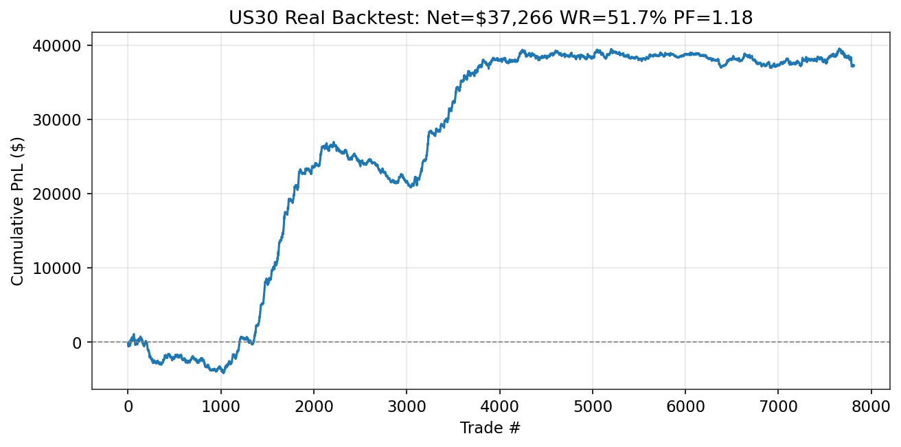
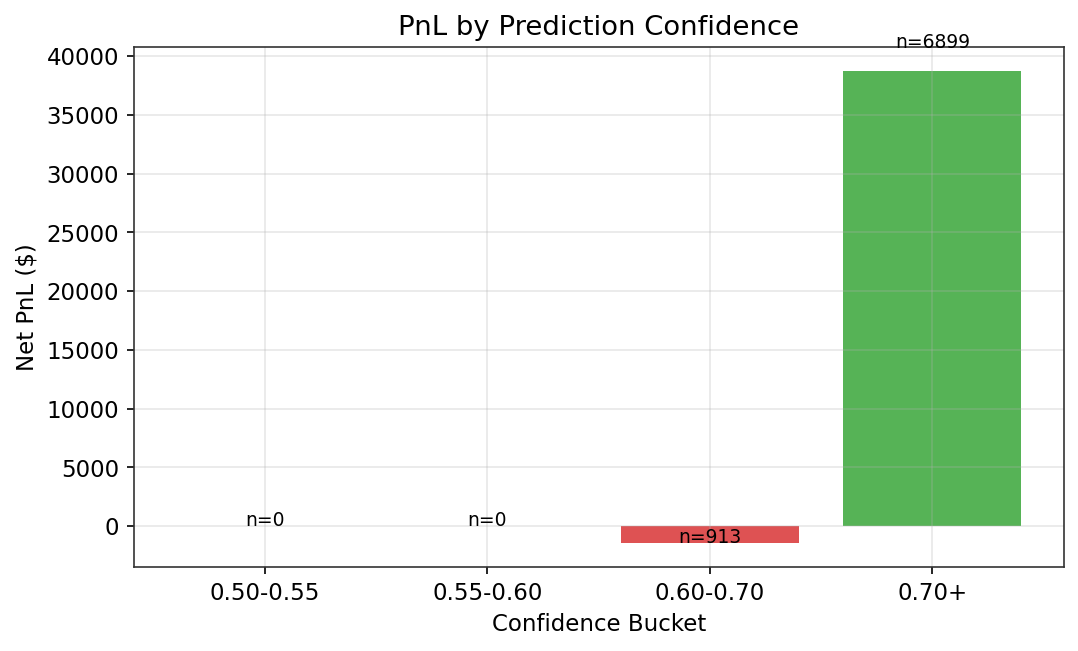
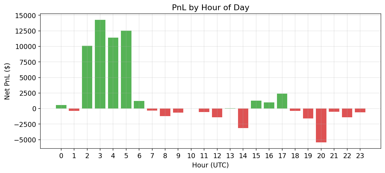
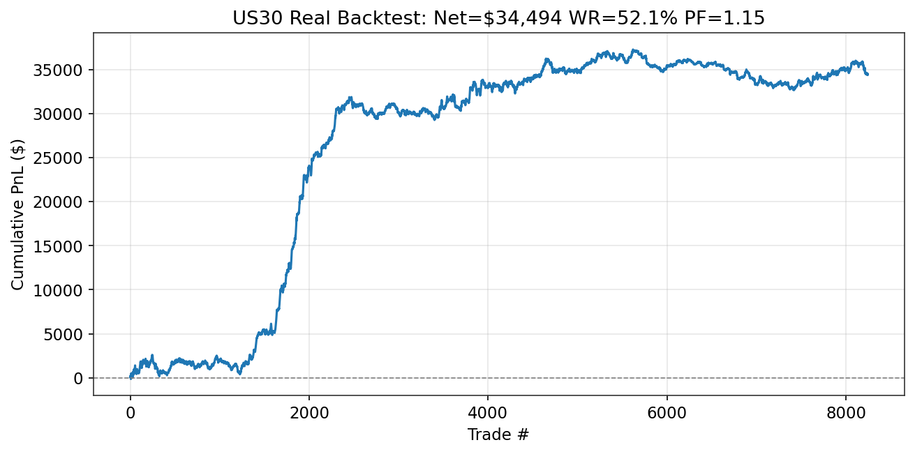
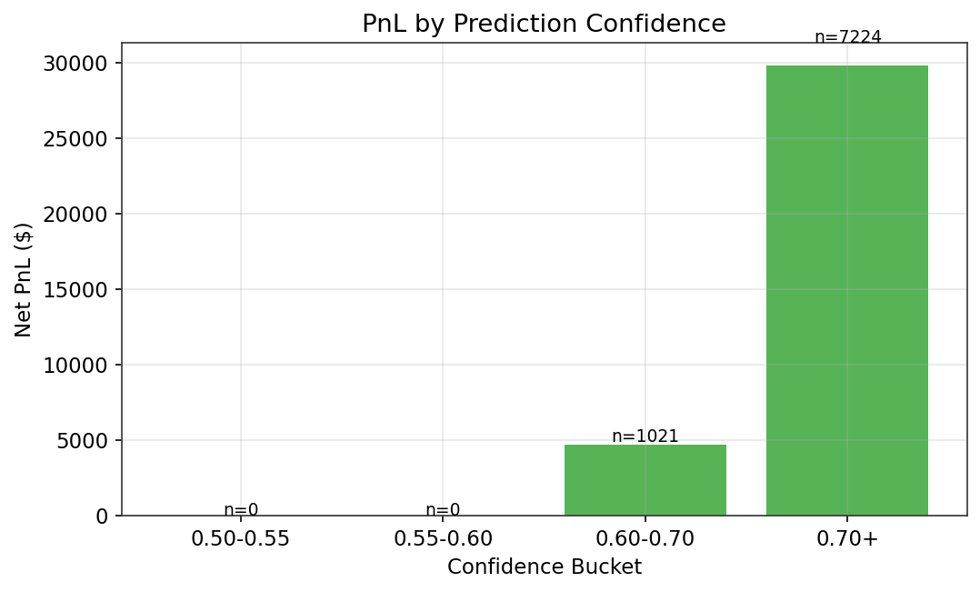
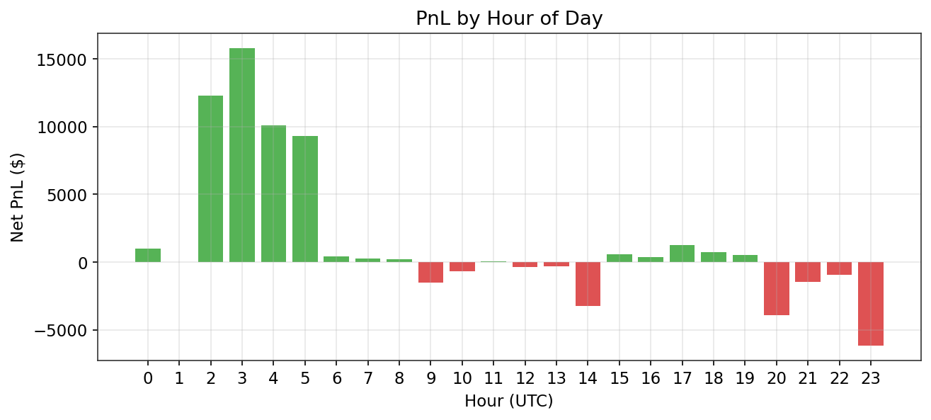
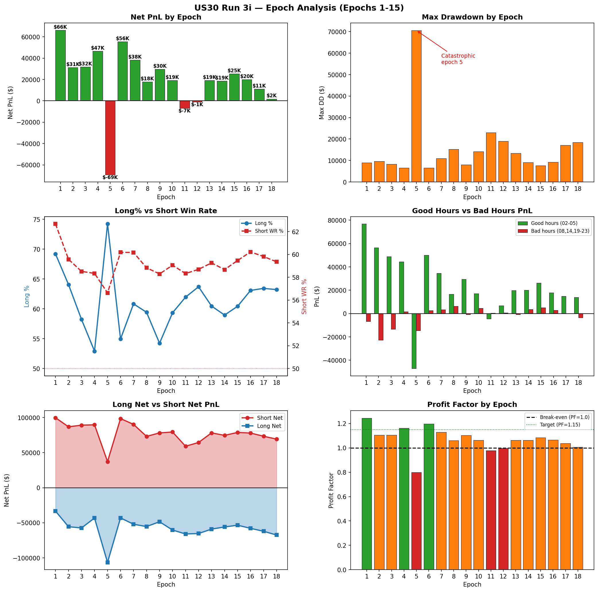
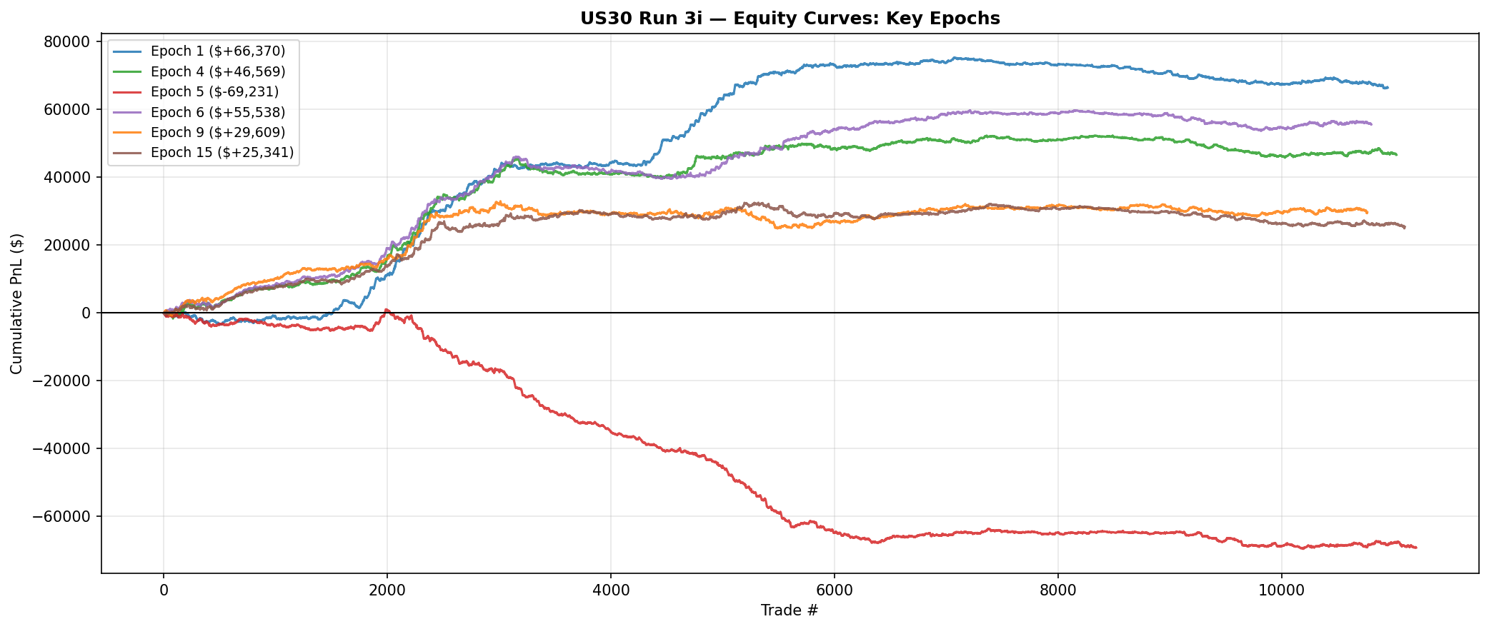
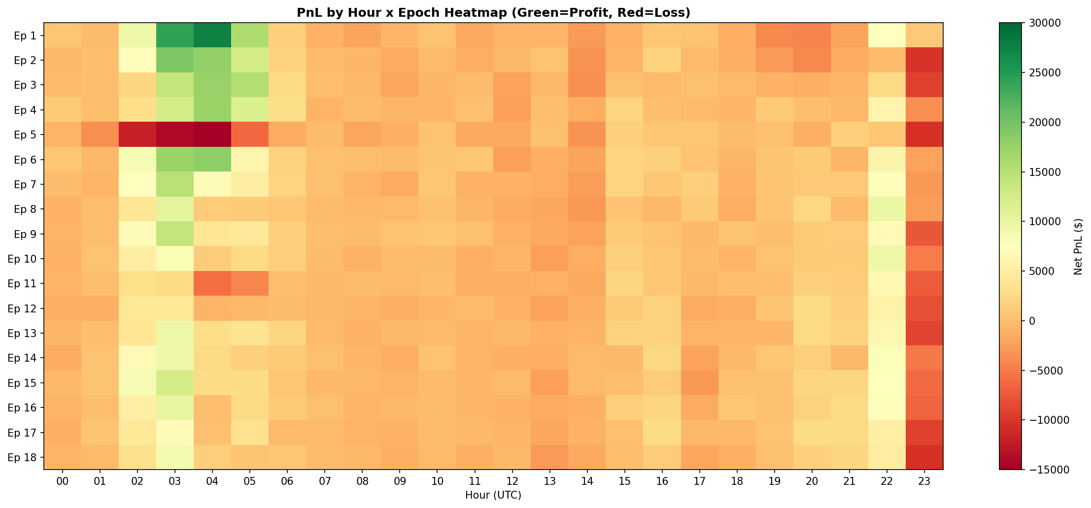
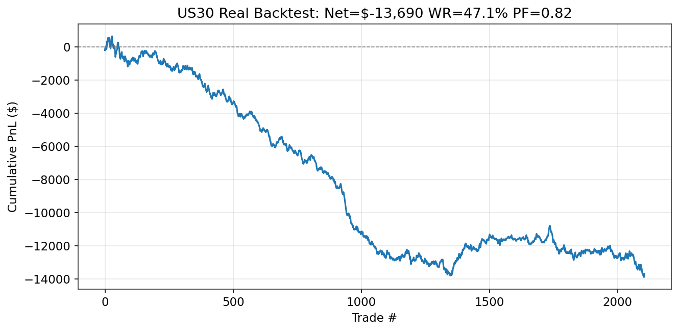
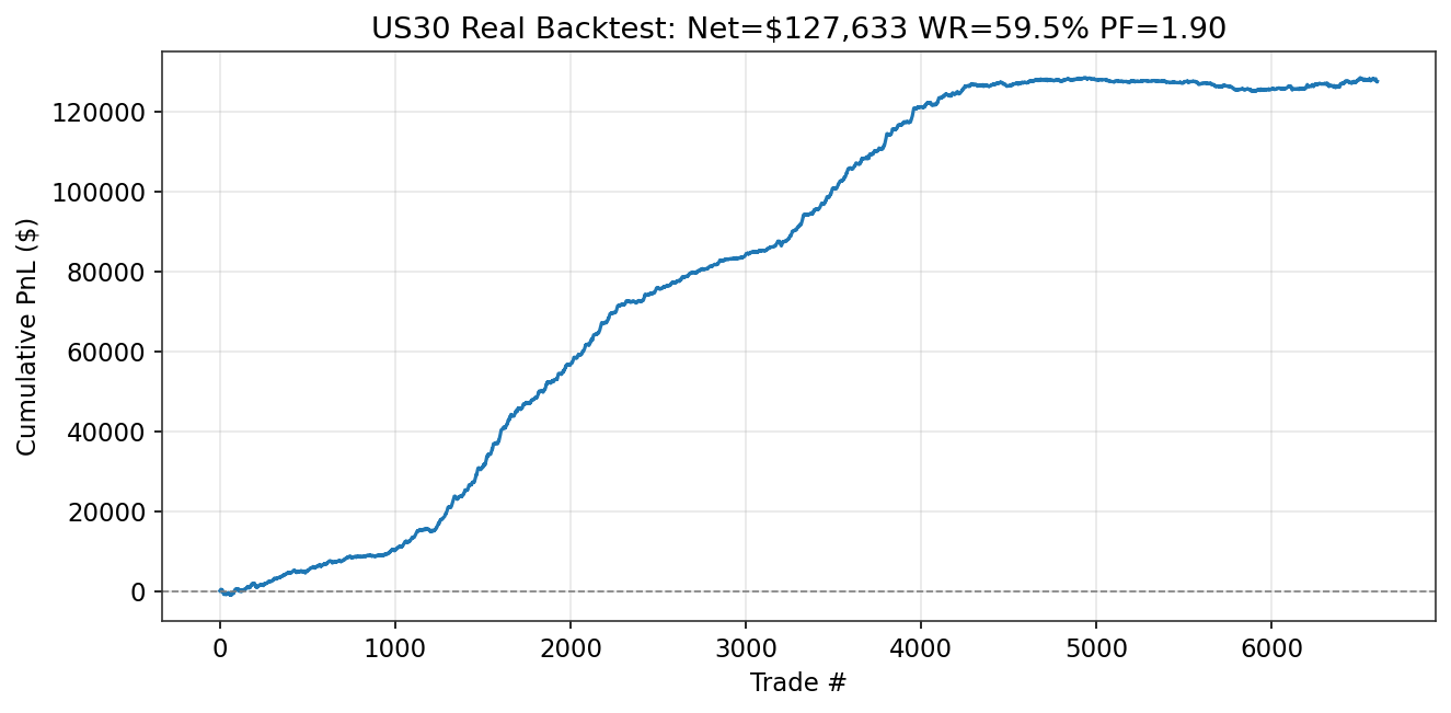
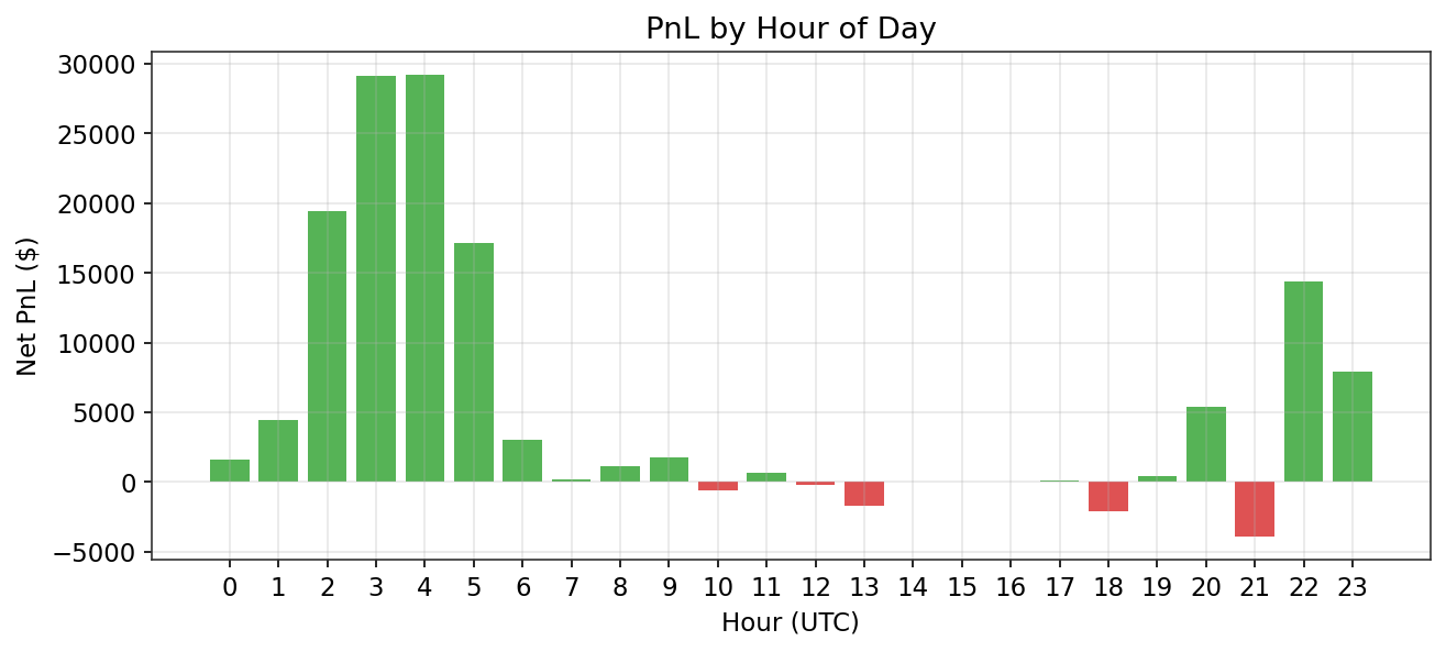
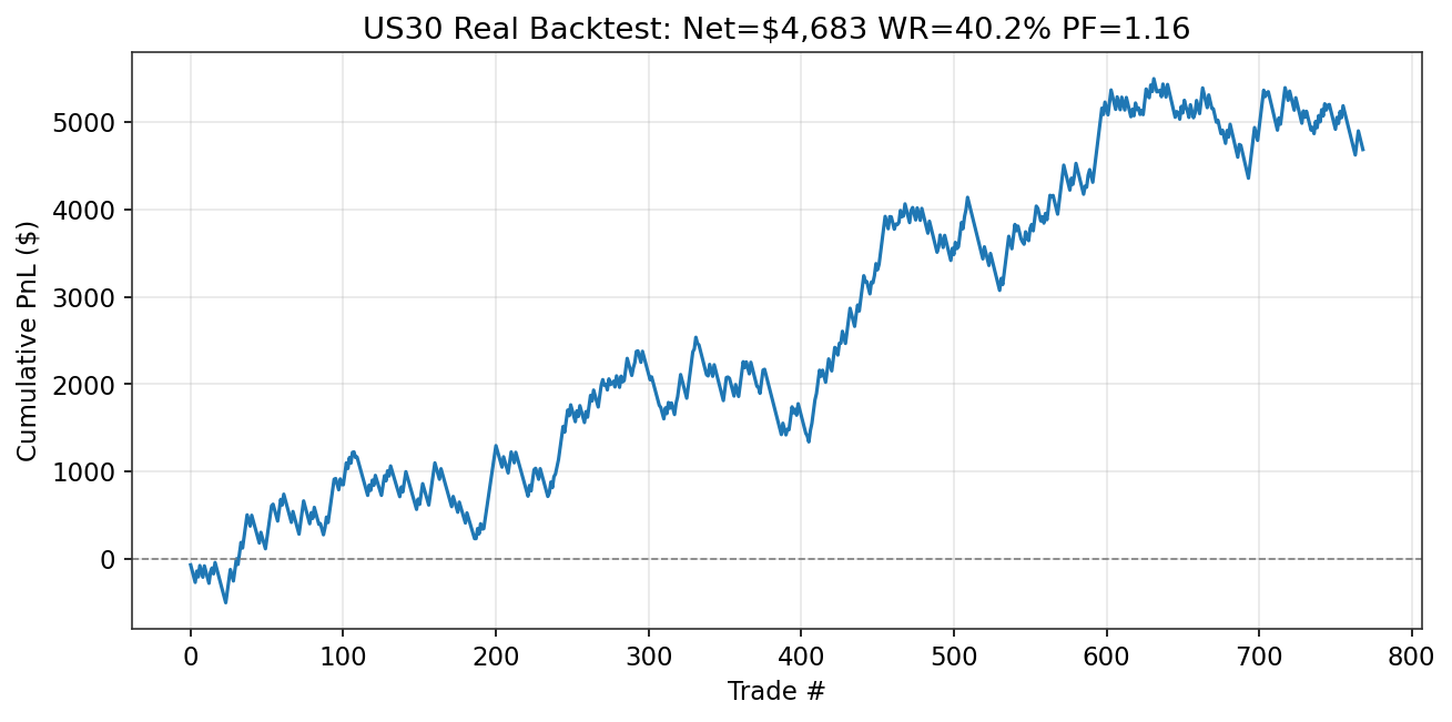
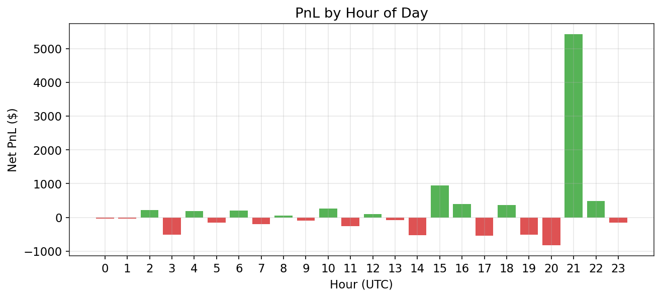
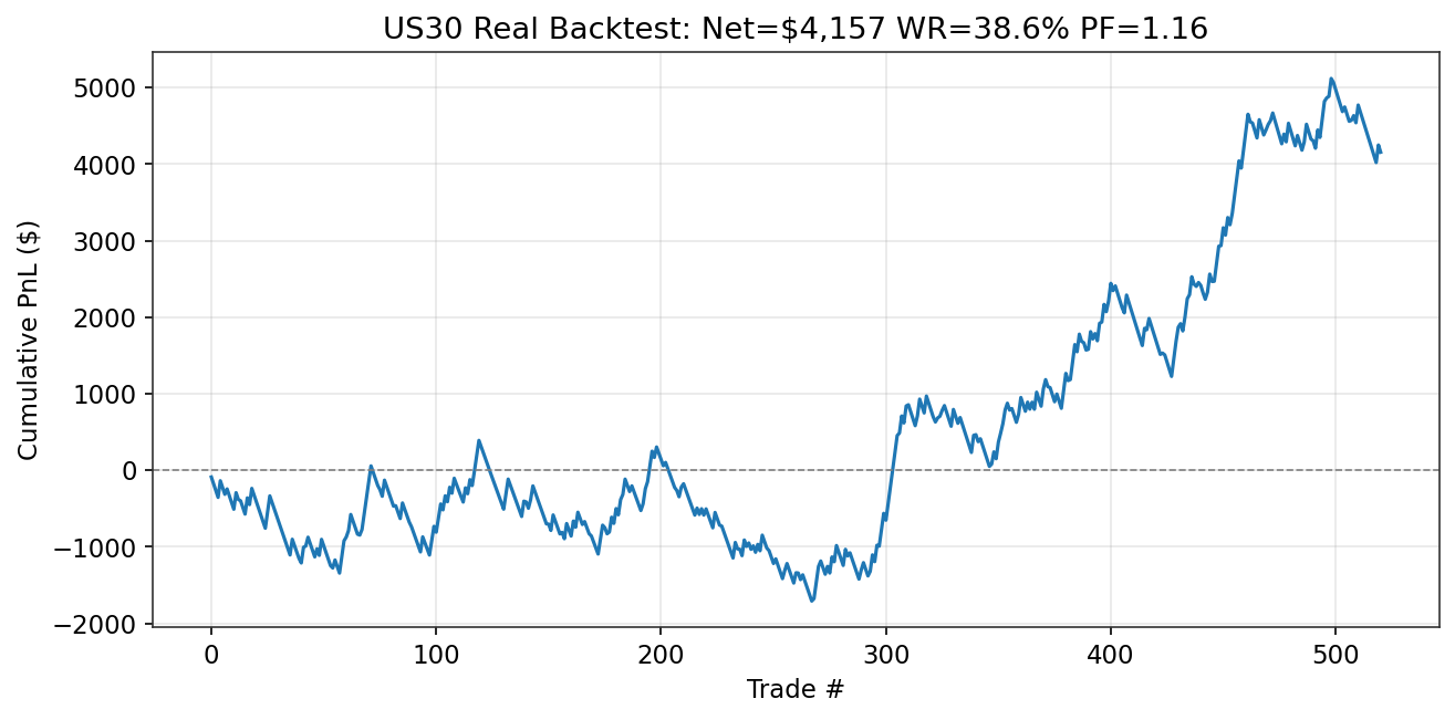
9. References

#	Authors	Year	Title	Venue
1	Lo, A.W. & MacKinlay, A.C.	1990	An Econometric Analysis of Nonsynchronous Trading	Journal of Econometrics
2	Chordia, T. & Swaminathan, B.	2000	Trading Volume and Cross-Autocorrelations in Stock Returns	Journal of Finance
3	Stoll, H.R. & Whaley, R.E.	1990	The Dynamics of Stock Index and Stock Index Futures Returns	J. Financial & Quantitative Analysis
4	Hasbrouck, J.	2003	Intraday Price Formation in U.S. Equity Index Markets	Journal of Finance
5	Huth, N. & Abergel, F.	2011	High Frequency Lead/Lag Relationships: Empirical Facts	arXiv:1111.7103
6	Engle, R.F.	2002	Dynamic Conditional Correlation	J. Business & Economic Statistics
7	Forbes, K.J. & Rigobon, R.	2002	No Contagion, Only Interdependence	Journal of Finance
8	Hamilton, J.D.	1989	A New Approach to the Economic Analysis of Nonstationary Time Series	Econometrica
9	Ang, A. & Bekaert, G.	2002	International Asset Allocation With Regime Shifts	Review of Financial Studies
10	Barberis, N. & Shleifer, A.	2003	Style Investing	J. Financial Economics
11	Moskowitz, T.J. & Grinblatt, M.	1999	Do Industries Explain Momentum?	Journal of Finance
12	Moskowitz, T.J., Ooi, Y.H. & Pedersen, L.H.	2012	Time Series Momentum	J. Financial Economics
13	Zhu, X.	2024	Examining Pairs Trading Profitability	Yale Economics Working Paper
14	Greenwood, R. & Sammon, M.	2023	The Disappearing Index Effect	Harvard Business School WP 23-025
15	Li	2025	Volatility Risk and Vol-of-Vol Risk: State-Dependent VIX-S&P Correlations	J. Futures Markets
16	Rothe, J.	2023	Dynamic Sector Rotation	SSRN WP #4573209
17	Mamais	2025	Explaining and Predicting Momentum Performance Shifts	J. Forecasting
18	Li, Chen & Liu	2025	High-frequency lead-lag in Chinese index futures	arXiv:2501.03171
19	Johansen, S.	1991	Estimation and Hypothesis Testing of Cointegration Vectors	Econometrica
20	Nasdaq	2020	A Tale of Three Crises in the Past Two Decades	Whitepaper
21	Nasdaq	2025	Understanding the DJIA: Price-Weighted vs. Cap-Weighted Attribution	Whitepaper
22	Lim, B., Arík, S.Ö., Loeff, N. & Pfister, T.	2021	Temporal Fusion Transformers for Interpretable Multi-horizon Time Series Forecasting	International Journal of Forecasting
23	Granger, C.W.J.	1969	Investigating Causal Relations by Econometric Models and Cross-spectral Methods	Econometrica
24	Pagonidis, A.S.	2014	The IBS Effect: Mean Reversion in Equity ETFs	NAAIM Wagner Award Paper
25	Connors, L. & Alvarez, C.	2009	Short Term Trading Strategies That Work	TradingMarkets
26	Collobert, R. & Weston, J.	2008	A Unified Architecture for Natural Language Processing	ICML 2008