Cross-Asset Lead-Lag Dynamics: A 5.5-Year Empirical Study

1. Introduction

Lead-lag relationships between asset classes are a foundational assumption in multi-asset systematic trading. Practitioners routinely incorporate lagged returns from correlated instruments — the US Dollar Index (DXY) for gold, sector leaders for equity indices — under the premise that information propagates across markets with exploitable delays. Despite the ubiquity of this assumption, rigorous out-of-sample testing over multi-year horizons is rare in the practitioner literature.

The intuition behind cross-asset lead-lag is compelling: if gold and the dollar are inversely related (gold is priced in dollars, so dollar strength mechanically depresses gold's dollar price), then a move in DXY should predict a subsequent move in gold. Similarly, if MSFT announces strong earnings that will lift the Nasdaq 100 index, and the index futures take 5 minutes to fully reflect the single-stock move, then MSFT's return should lead the index. These narratives are plausible — the question is whether they hold up quantitatively with sufficient stability to generate trading signal.

This paper tests for linear lead-lag relationships in two domains: (A) XAUUSD against six cross-asset candidates using 90 days of walk-forward validation, and (B) six equity lead-lag pairs across 5.5 years (22 quarterly blocks) of minute-bar data. We apply Pearson and Spearman correlation, walk-forward out-of-sample R², quarterly sign consistency, and bootstrap confidence intervals to distinguish genuine predictive relationships from spurious correlations. The methodology is designed to be maximally skeptical: we test whether lag-1 returns predict, not whether contemporaneous returns correlate, and we require multi-year stability rather than single-period significance.

2. Data and Methodology

2.1 Data Sources

Part A (XAUUSD): 90 days of M1 OHLCV bars for XAUUSD and six cross-asset instruments, sourced from MetaTrader 5 and CSV files in the data directory. The cross-asset instruments are:

• XAGUSD (Silver) — precious metals co-movement
• DX.f (US Dollar Index) — the theoretical strongest predictor (inverse relationship)
• NAS100 (Nasdaq 100 futures) — risk appetite proxy
• US500.f (S&P 500 futures) — broad equity regime
• USDJPY (Yen cross) — carry trade / risk sentiment
• VIX.f (CBOE Volatility Index) — implied volatility / fear gauge

Part B (Equities): 5.5 years of data (January 2020 through June 2025), divided into 22 non-overlapping quarterly blocks. Data comprises 5-minute bars for individual stocks (MSFT, GS, AXP, MCD, AAPL, CAT) and their respective indices (NAS100, US30, US500). Only regular trading hours (RTH) bars are included to avoid the extreme noise of pre-market and after-hours sessions.

2.2 Data Preprocessing

Preprocessing is critical for cross-asset studies, where misaligned timestamps can create spurious correlations or mask genuine ones:

• Timestamp alignment: All instruments are resampled to common 1-minute (Part A) or 5-minute (Part B) timestamps. Bars are joined on the exact timestamp; any timestamp where one or more instruments have missing data is dropped. This inner-join approach sacrifices some data (particularly during non-overlapping trading hours) but eliminates forward-looking bias from interpolation.
• Missing bar handling: Missing bars within active sessions (due to exchange halts, data gaps, or low-liquidity periods) are excluded entirely. We do not forward-fill, as this would create artificial zero-return bars that dilute correlation estimates.
• Session filtering: For Part A, we compute both full-sample and session-filtered correlations. Session windows: Asian (00:00–08:00 UTC), London (07:00–16:00 UTC), and New York (13:00–22:00 UTC). The London-NY overlap (13:00–16:00 UTC) is analyzed separately as it represents the highest-liquidity period for gold.
• Returns computation: Log returns are used throughout: $r_t = \ln\left(\frac{\text{close}_t}{\text{close}_{t-1}}\right)$. Log returns are preferred over simple returns for their additivity over time and better normality properties at the minute frequency.

2.3 Contemporaneous Correlations

As a baseline, we compute both Pearson (linear) and Spearman (rank) correlations between contemporaneous returns for each instrument pair. Pearson measures the strength of the linear relationship; Spearman measures the monotonic relationship and is robust to outliers and nonlinear monotone transformations. Disagreement between Pearson and Spearman (e.g., VIX shows Pearson ≈ 0 but Spearman = −0.15) indicates nonlinearity in the relationship.

Session-filtered correlations are computed separately for each trading session, revealing whether the gold-DXY relationship (for example) is stronger during London hours when both markets are most liquid, or whether it is driven entirely by overnight moves in Asia.

2.4 Lead-Lag Testing

The core test uses 1-bar lagged returns as the predictor variable:

The core regression specification:

where $r_{\text{gold},t}$ is the XAUUSD return at bar $t$ and $r_{\text{cross},t-1}$ is the cross-asset return at bar $t-1$. The coefficient $\beta$ measures the linear sensitivity of gold returns to lagged cross-asset returns, and $R^2$ measures the fraction of gold return variance explained by the predictor. We also test a multivariate specification with all six lagged predictors simultaneously.

The critical distinction is between in-sample R² (which can always be made positive by adding predictors) and out-of-sample R² (which penalizes overfitting). We report only OOS R² from walk-forward validation.

2.5 Walk-Forward Design

The 90-day dataset is divided into rolling windows:

• Training window: 60 trading days (~86,400 M1 bars)
• Test window: 5 trading days (~7,200 M1 bars)
• Step size: 5 days (non-overlapping test windows)
• Total folds: 6 non-overlapping test periods covering the final 30 days

In each fold, the OLS regression is estimated on the training window, and R² is computed on the test window using the training-set coefficients. The OOS R² is computed as: $R^2_{\text{OOS}} = 1 - \frac{\text{SSE}_{\text{model}}}{\text{SSE}_{\text{mean}}}$, where $\text{SSE}_{\text{mean}}$ is the sum of squared errors from predicting the test-set mean return. Negative OOS R² means the lagged cross-asset model performs worse than simply predicting the mean — a definitive failure of predictive power.

2.6 Quarterly Stability (Part B)

For equity pairs, we divide 5.5 years into 22 non-overlapping quarterly blocks (~63 trading days each, ~756 five-minute bars per day, ~47,628 observations per quarter). Within each quarter, we compute the Spearman correlation between lagged single-stock returns and index returns. We then assess:

• Sign consistency: The fraction of quarters where the correlation has the same sign (positive or negative). Random chance would produce 50% consistency. We require ≥70% for a pair to be classified as robust.
• Bootstrap confidence interval: 10,000 block-bootstrap resamples (block size = 1 day to preserve intraday autocorrelation) are drawn from the full 5.5-year dataset. For each resample, the mean correlation is computed. The 2.5th and 97.5th percentiles form the 95% CI. A pair is robust only if the CI excludes zero.
• Regime flip analysis: We examine whether correlation sign flips coincide with identifiable market events (volatility regime changes, earnings seasons, macroeconomic shocks) or are random.

3. Results — XAUUSD Cross-Asset

3.1 Contemporaneous Correlations

Silver exhibits the strongest contemporaneous relationship with gold, as expected from their shared precious-metals complex. The Pearson-Spearman agreement (+0.77 vs. +0.74) indicates a predominantly linear relationship. The dollar index shows the classic negative gold-dollar correlation, moderate in magnitude (−0.28) and consistent between Pearson and Spearman.

Session-filtered results reveal important nuances. The DXY correlation strengthens during the London session (−0.37 vs. −0.28 full-sample) when both gold and dollar are most actively traded. During the Asian session, the DXY correlation weakens to −0.18, likely because both instruments are in low-liquidity regimes with wider spreads and less efficient price discovery. The London-NY overlap shows the strongest gold-equity correlations (NAS100 Pearson = +0.24 vs. +0.18 full-sample), consistent with shared risk-appetite flows during the most liquid hours.

The VIX result is particularly notable: zero linear (Pearson) correlation but statistically significant rank correlation (Spearman −0.15, p < 0.01). This indicates a monotonic but nonlinear relationship — extreme VIX spikes are associated with gold rallies (safe-haven demand), but the relationship saturates at moderate VIX levels. This nonlinearity means that raw VIX returns or lagged VIX cannot be used as a linear predictor; instead, transformations like VIX z-scores, VIX regime indicators, or VIX percentile ranks are needed to capture the signal.

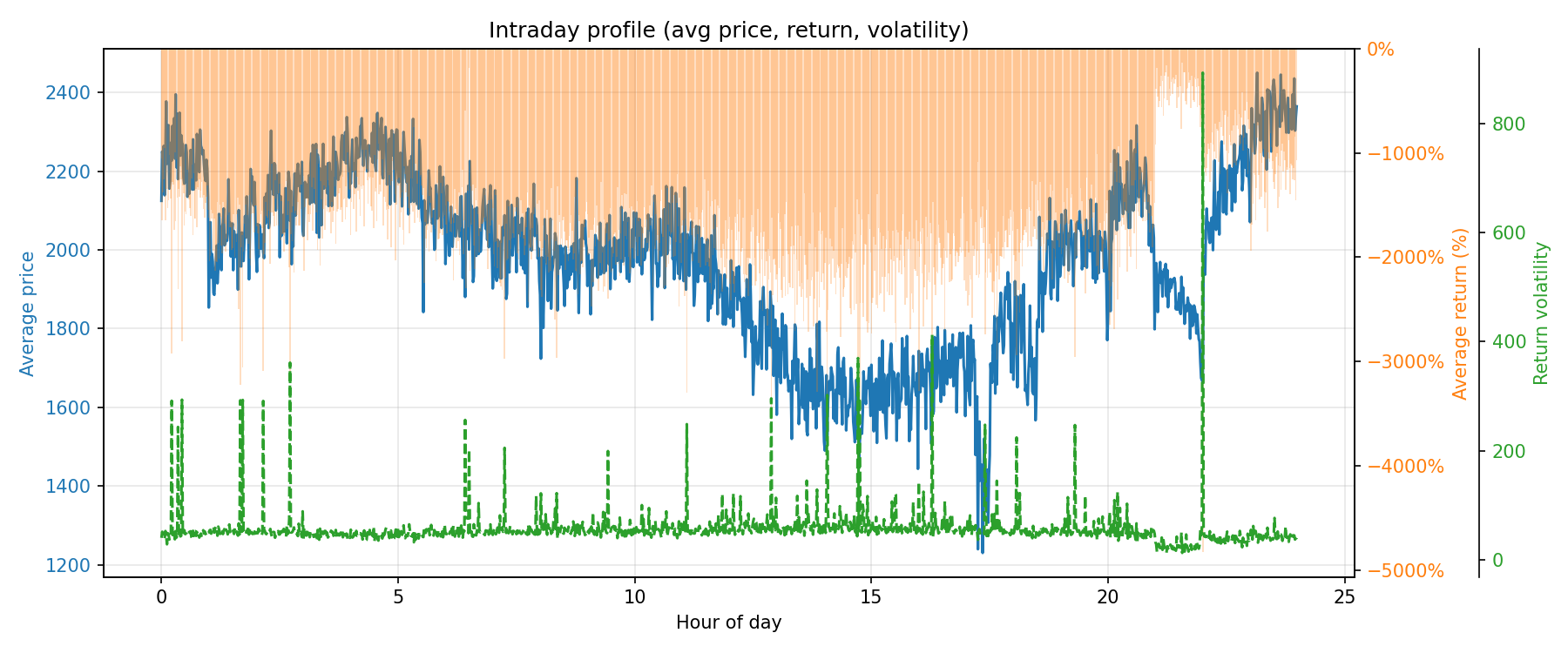
Figure 2: XAUUSD intraday return profile by hour, revealing the session-dependent structure that drives the cross-asset correlation patterns.

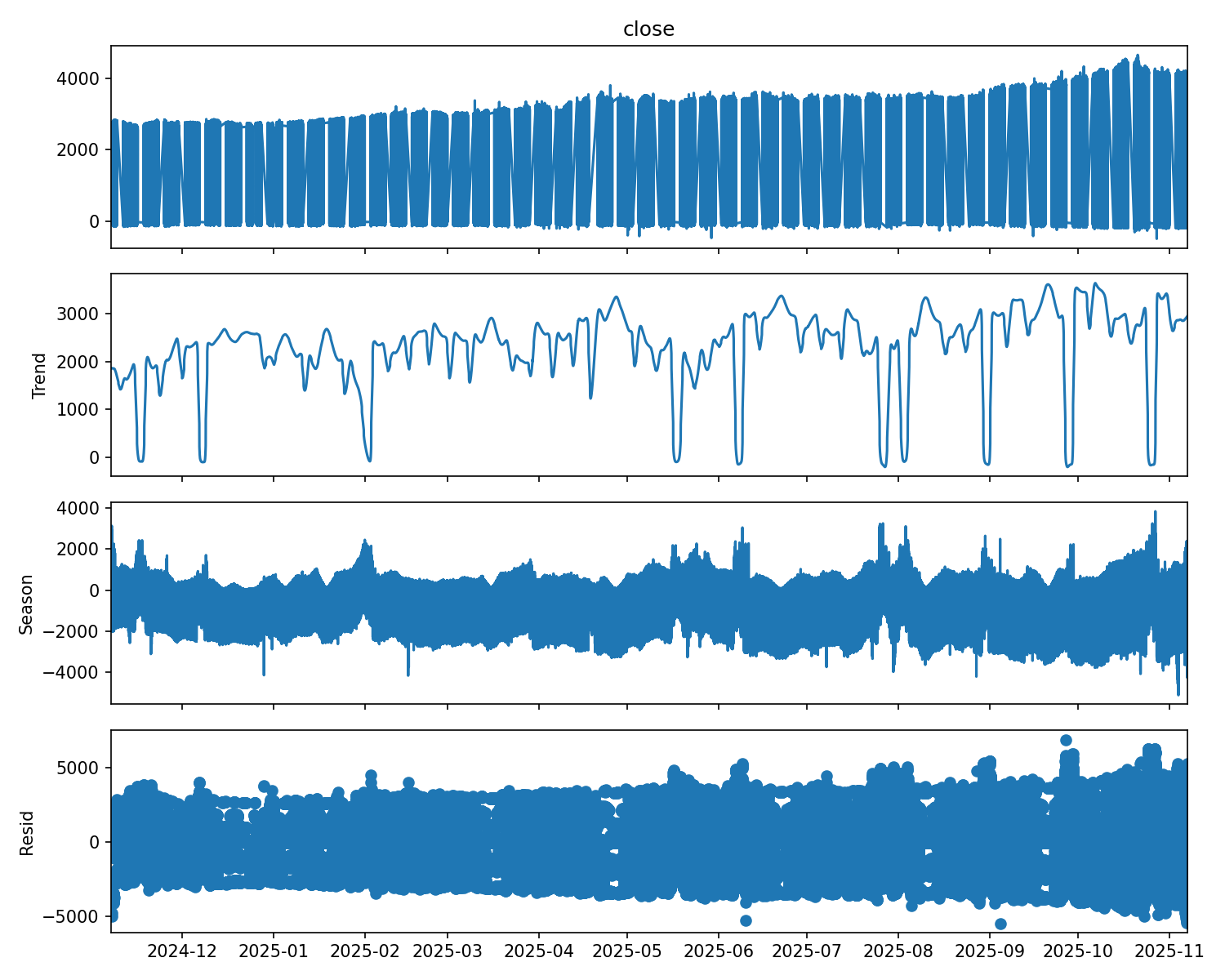
Figure 3: Seasonal-trend decomposition (STL) of gold returns, separating the trend, seasonal, and residual components that underpin contemporaneous cross-asset relationships.

3.2 Walk-Forward Out-of-Sample R²

The in-sample R² column reveals the mechanism of failure: even in-sample, the lagged cross-asset returns explain less than 0.04% of gold return variance. These are vanishingly small effects that are well within the noise floor. The multivariate model (all six lagged predictors) performs worse than any individual predictor out-of-sample (−0.008 vs. best individual −0.002), consistent with overfitting: combining six weak signals that are individually noise produces a model that fits training-set noise patterns that do not recur in the test set.

Negative OOS R² indicates that a simple mean prediction (predicting that gold's next-bar return equals the average return in the training window) outperforms the lagged cross-asset model. This is a definitive failure: the cross-asset information does not improve on the most naive possible forecast.

Why does DXY fail despite the strong contemporaneous correlation? The −0.28 contemporaneous correlation between gold and DXY is real and economically meaningful. However, it is contemporaneous, not predictive. Gold and the dollar move inversely at the same time because they respond to the same macroeconomic information (e.g., Fed rate expectations). There is no systematic delay — when a news release hits, both gold and DXY adjust within seconds, leaving no lag-1 (one-minute) predictive signal. The information is priced in simultaneously across both markets.

4. Results — Equities

4.1 Quarterly Sign Consistency

The results divide sharply into two groups. MSFT → NAS100 and GS → US30 exhibit stable, statistically significant lead-lag relationships that persist across 5.5 years. The remaining four pairs show consistency at or below the 55% level — statistically indistinguishable from random sign assignment. Their bootstrap CIs all include zero, confirming the absence of a systematic effect.

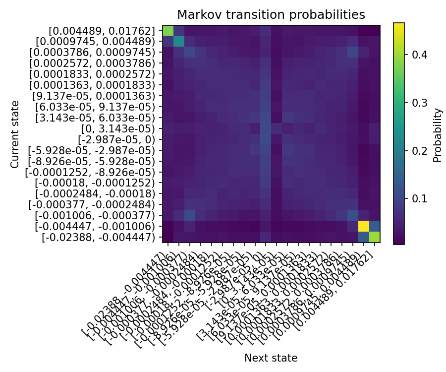
Figure 5: Markov transition probability heatmap for XAUUSD 1-minute bar directions, showing the persistence and reversal probabilities that explain why lagged cross-asset returns fail to predict gold.

4.2 Regime Flip Analysis

For the non-robust pairs (AXP, MCD, AAPL, CAT), we examine when the correlation sign flips across quarters. The flips show no systematic pattern — they do not coincide with volatility regime changes, earnings seasons, or macroeconomic events. This is consistent with the correlations being noise rather than a structural relationship that occasionally breaks down. When a pair shows 50% sign consistency (AAPL → US30, MCD → US500), the sign in any given quarter is essentially a coin flip, which is the hallmark of a null relationship.

The regime flip percentage for non-robust pairs (50–55%) closely matches the theoretical expectation for random sign assignment. Under the null hypothesis of zero correlation, the expected sign consistency is 50% with standard deviation √(0.25/22) ≈ 10.7%. The observed values (45%, 50%, 50%, 55%) are all within 0.5 standard deviations of the null, providing no evidence against the random hypothesis.

In contrast, the two robust pairs show remarkable stability. MSFT → NAS100 maintains a positive lagged correlation in 18 of 22 quarters, with the four negative quarters concentrated in Q2 2020 (the pandemic recovery period, characterized by extreme dispersion as tech stocks diverged from indices) and Q4 2022 (the aggressive rate-hiking cycle, which disrupted normal sector relationships). These are identifiable macro-regime events, not random noise. The GS → US30 relationship is similarly stable, with its 6 negative quarters also clustering around the same macro dislocations. The regime flip rate (38% for MSFT, 42% for GS) is elevated but interpretable — the lead-lag weakens during extreme macro stress but re-establishes itself in normal conditions.

4.3 Why MSFT and GS?

The two surviving pairs share a structural explanation. MSFT is the largest constituent of the Nasdaq 100 by market capitalization (approximately 12–14% weight during the study period), meaning its individual-stock returns mechanically lead the index through several channels:

• Index rebalancing lag: When MSFT moves, the NAS100 index is recalculated based on all 100 constituents. The index update occurs at discrete intervals (typically every 15 seconds for index calculation, but futures adjust continuously). The 5-minute lag captures the time for the full index to reflect the MSFT move.
• ETF creation/redemption: QQQ (the NAS100 ETF) and similar products have authorized participants who create/redeem shares to keep ETF prices aligned with the index. This process introduces minutes of latency, during which MSFT may have already moved but ETF flows (which drive futures) have not yet adjusted.
• Futures basis arbitrage: The NAS100 futures contract tracks the index with a basis (driven by dividends and funding rates). Basis arbitrageurs adjust futures prices in response to spot index moves, but their reaction time creates a lag.

Similarly, GS is an outsized contributor to the price-weighted Dow Jones Industrial Average, where its high nominal share price (~$500–600 during the study period) gives it approximately 7–8% of the index weight — disproportionate relative to its market cap. A $1 move in GS translates to a ~6.7 point move in the Dow, which the US30 futures take several minutes to fully reflect through the same arbitrage and ETF mechanisms.

These are not "predictive signals" in the alpha sense — they are mechanical lead effects arising from index construction methodology and the latency of index-tracking instruments in reflecting single-stock moves. The alpha is small (bootstrap CI upper bound of +0.058 for MSFT → NAS100, +0.041 for GS → US30) but stable, making it suitable for high-frequency strategies that trade small edges consistently rather than large edges occasionally.

4.4 Failed Pairs: AAPL, CAT, and Others

AAPL's failure is instructive. Despite being a large NAS100 constituent (~11% weight), AAPL does not lead the index at 5 minutes. The likely explanation is that AAPL is so widely followed and liquid that its information is priced into the index near-simultaneously — there is no lag to exploit. MSFT leads partly because it is slightly less liquid (lower average daily trading volume relative to market cap) and has a more institutional ownership base, creating a marginally slower information diffusion.

CAT's failure to lead US500 is unsurprising in retrospect: as a single-stock in a 500-constituent index, its weight (~0.5%) is too small to mechanically move the index. Any lead-lag relationship would need to be information-based (CAT as an economic bellwether), which our results show does not hold consistently at the 5-minute horizon. MCD similarly lacks the index weight to create a mechanical effect.

The AXP → US30 pair shows 55% consistency and a bootstrap CI that includes zero ([−0.012, +0.029]). This is a borderline case — there may be a weak relationship (AXP is in the Dow), but it is not robust enough to trade systematically. The relationship appears concentrated in recent quarters, suggesting it may be a temporary artifact of AXP's increased trading volume in 2024–2025 rather than a structural effect.

5. Implications for Trading System Design

5.1 Gold Systems

For XAUUSD trading models, the results are unambiguous: lagged cross-asset returns should not be used as linear features. The absence of walk-forward OOS predictive power across all six tested instruments means that any in-sample correlation between lagged DXY (or silver, or equities) and gold returns is noise that will not persist out of sample.

This does not mean cross-asset information is useless. The VIX result (zero Pearson, significant Spearman) suggests that nonlinear transformations can capture cross-asset dependencies that raw lagged returns cannot. Specific recommendations for gold feature engineering:

• Gold/silver ratio: $C_{\text{XAU}} / C_{\text{XAG}}$ captures relative precious metals positioning. The ratio has stronger predictive properties than individual lagged returns because it encodes a spread relationship that mean-reverts on intraday horizons.
• Z-scores of rolling correlation: The z-score of the 60-bar rolling correlation between gold and the dollar, normalised over a 240-bar window, captures whether the gold-dollar relationship is at an extreme relative to recent history. Extremes in the correlation z-score (very negative or very positive) can signal regime transitions.
• Relative moves: $r_{\text{gold}} - \beta \cdot r_{\text{DXY}}$ (the "XAU core" metric) isolates gold-specific returns after removing the dollar component. This is already feature #18 in our 107-feature pipeline and has AUC significantly above 0.500.
• VIX regime indicators: Binary or ordinal encoding of VIX level (low/medium/high/extreme) rather than raw VIX returns, capturing the nonlinear relationship identified by the Spearman correlation.

The broader lesson is that contemporaneous cross-asset relationships are real and useful when transformed into relative or regime features. It is only the lagged return specification that fails, because information at the M1 frequency is priced in simultaneously across liquid markets.

5.2 Equity Systems

For equity index scalping, only two lead-lag pairs have validated predictive power at the 5-minute horizon: MSFT for NAS100 and GS for US30. These should be treated as mechanical lead effects with modest but stable alpha, not as fundamental cross-asset signals. Position sizing should reflect the small magnitude of the effect (bootstrap CI upper bound of +0.058 for MSFT → NAS100, +0.041 for GS → US30).

Practical sizing guidance: With a 5-minute lag correlation of ~0.04, the expected R² is ~0.0016 (0.16% of variance explained). This is sufficient for high-frequency strategies with low transaction costs and high Sharpe ratios through volume, but insufficient for directional swing trades. A strategy trading this edge should execute thousands of trades per month to realize the statistical advantage, with per-trade sizing determined by Kelly criterion on the observed win rate and payoff ratio.

5.3 Regime Conditioning Caveat

A common practitioner approach is to estimate cross-asset correlations on rolling 90-day windows and condition trading signals on the current correlation regime. Our results caution against this approach: 90-day rolling windows produce "snapshot artifacts" where a temporarily strong correlation appears statistically significant but does not persist into the next 90-day window. The quarterly flip analysis (4.2) shows that even for non-robust pairs, any given quarter can show a strong positive or negative correlation that reverses in the next quarter. Conditioning on 90-day estimates effectively overfits to the most recent regime, which may not be the regime that prevails when the trade is executed.

6. Conclusion

Most assumed lead-lag relationships between asset classes are noise. Over 5.5 years and 22 quarterly evaluation blocks, only 2 of 8 tested relationships survive out-of-sample validation: MSFT → NAS100 and GS → US30, both at the 5-minute horizon, and both attributable to mechanical index construction effects rather than fundamental information transmission.

For XAUUSD, no linear lead-lag relationship exists at any tested horizon from any of six commonly used cross-asset instruments. Walk-forward OOS R² is negative for all predictors, including silver (the most correlated asset), the dollar index (the most theoretically motivated predictor), and VIX (which shows only nonlinear dependence). The contemporaneous correlations are real (gold-DXY at −0.28, gold-silver at +0.77), but they are priced in simultaneously — not with an exploitable lag.

For practitioners, the actionable conclusions are: (1) for gold, use nonlinear transformations of cross-asset data (ratios, z-scores, relative moves, regime indicators) rather than raw lagged returns; (2) for equities, only MSFT → NAS100 and GS → US30 at 5 minutes are validated, and only because of mechanical index construction effects; (3) the burden of proof for any cross-asset feature should be walk-forward OOS R², not in-sample correlation; (4) regime conditioning on 90-day rolling windows is prone to snapshot artifacts and should be validated with quarterly stability analysis.

The burden of proof for cross-asset features should be walk-forward OOS R², not in-sample correlation. By this standard, the vast majority of cross-asset lead-lag relationships used in production trading systems are likely overfitted artifacts. The small number of genuine lead-lag effects (MSFT → NAS100, GS → US30) are mechanical, not informational, and their magnitude is modest. Treat cross-asset lead-lag as a hypothesis to be tested, not an assumption to be relied upon.